A Comprehensive Exploration of Pooling in Neural Networks: A Python demo to Pooling in CNN

Machine Learning (ML) is the new buzz word of the 21st century and is the base of A.I. and computer intelligence. ML uses predictive models that learn the pattern from data to infer future trends or outcomes. Deep Learning is a sub-domain of ML, where the model is inspired by the neural network of the human brain. These models are capable of understanding the complex relationships between the inputs and the outputs. Deep Learning is the emerging approach and has been widely applied in the field of Natural Language Processing, Transfer Learning, Computer Vision and many more.

In this article, we will examine the Convolutional Neural Network (CNN), and dive deep to understand the concept of pooling to show why it is used in CNNs. We have also included a code demo that creates a CNN to classify objects from the CIFAR10 dataset. In the concluding section of the article, we will explore some emerging trends in pooling layers aimed at addressing the drawbacks associated with traditional pooling techniques.

Introduction to CNNs

A Convolutional Neural Network (CNN) is a specialized type of Deep Neural Network (DNN) comprising multiple convolution layers, each comprising an activation function and a pooling layer. This DNN is mostly used in object detection, classification or segmentation. A Convolutional Neural Network (CNN) is designed to analyze and classify input images into various predefined classes.

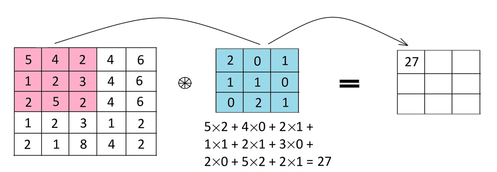
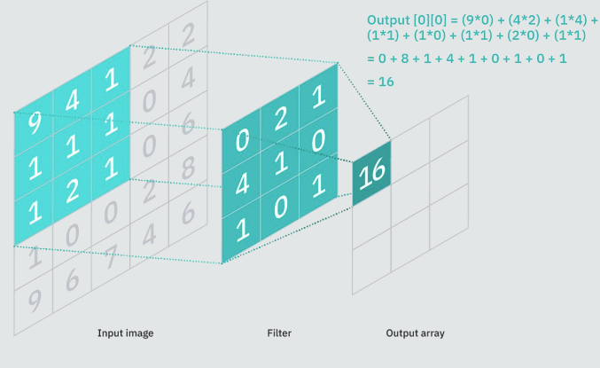
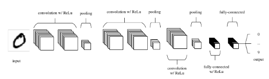
The image undergoes a sequential process involving different layers, including convolutional layers, pooling layers, and fully connected layers. The convolution layer uses specific filters (kernels) to extract features from an image. A filter in simpler terms is a feature detector. Hence, specific filters are used to detect specific features in an image. This filter is applied to the input data or image by sliding it over the entire input. At each cell element wise multiplication is carried out, and results are summed up to produce a single value for that specific cell. Furthermore, the filter takes a stride jump and the same operation is repeated until the entire image is captured. The output of this operation is known as a feature map.

Feature maps are responsible for capturing specific patterns depending on the filter used. As the filter takes the stride jump across the input, it detects different local patterns, capturing spatial information.

This operation is known as Convolution operation in CNN. Convolutional layers are crucial in image-related tasks because they allow the network to automatically learn.

To understand the Convolution operation in detail, feel free to check out some of our other tutorials, like this one or this one, on the Paperspace Blog.

The pooling layer is usually added after the convolution layer. An effective pooling method is expected to selectively extracting relevant information while discarding irrelevant details.

Purpose of Pooling in Deep Learning

Pooling is a technique used in Convolutional Neural Networks (CNNs) to downsample the spatial dimensions of the input feature maps, reducing the amount of computation and parameters in the network while retaining important information. Pooling is typically applied after convolutional layers and before fully connected layers in a CNN. Pooling layers are typically applied to learn invariant features. In simpler terms, the pooling layer takes in the output from the convolution layer and retains the important information of the input image and discards the information which is unnecessary. This helps in reduction of the dimensionality of the feature map.

Pooling leads to a significant reduction in the spatial dimensions of the input, serving two primary objectives. Firstly, it diminishes the number of parameters or weights, thereby lowering computational costs. Secondly, it helps control overfitting in the network because there are less parameters. Another advantage of pooling is it makes the ML model more robust to object positions in image as pooling makes the model tolerant towards variations or image distortions.

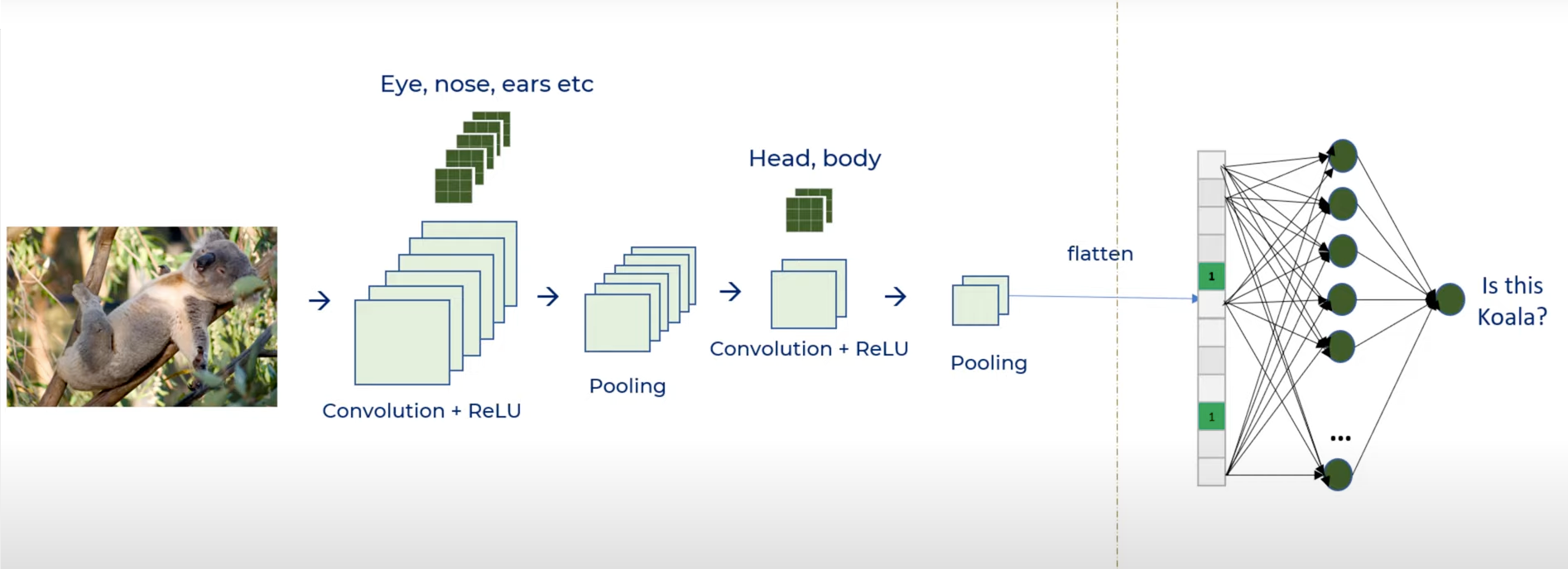
Few of the most common pooling methods which are widely used are Average Pooling, Max Pooling, Min Pooling, Mixed Pooling, Global Pooling, 𝑳𝑷 Pooling and few of the novel pooling methods includes Multi-scale order-less pooling (MOP), Super-pixel Pooling, and Compact Bilinear Pooling. The below image shows how CNN works for detecting an object in an image.

How does Pooling work?

Pooling works quite similar to convolution operation, pooling requires a certain filter and this filter slides over the feature map (output) obtained using the convolution operation.

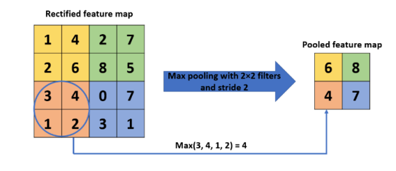
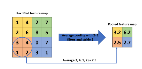
A sliding window moves across the feature map during pooling. This sliding window defines regions where the pooling function is applied, and the output value generated within each region replaces the original values contained in that specific area. Similar to a convolution operation, this process is repeated until the entire feature map is processed. Unlike in convolution, pooling lacks weights; instead, it utilizes pooling operations that generate a single value as the output. The specific pooling operation chosen determines how this calculation is performed. In the majority of cases, either Max-Pooling or Average Pooling is used. Max pooling grabs the largest value, while Average Pooling calculates the average value to use.

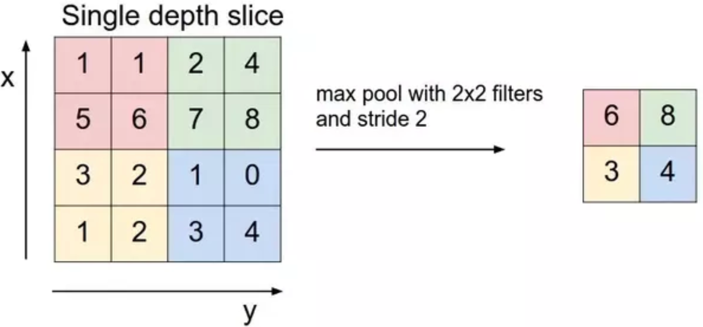
Often, a 2×2 filter is employed and moved across the input with a stride of 2. This implies that the pooling layer reduces the size of the feature map by a factor of 2. In simpler terms, each dimension becomes half of its previous size, resulting in each feature map value being reduced to one-quarter of its original size. For instance, if the initial feature map is [4×4], the applied pooling layer would output a feature map of size [2×2]. Similarly, a feature map of [16x16x10], with a filter of [2x2] and a stride of 2, would yield an output of [8x8x10].

Most of the time, convolutions and pooling layers are stacked alternatively all the way until the size of the output feature map shrinks. This output then gets fed into a fully connected neural network. 

There are several frameworks which can be used to implement pooling in CNN. Tensorflow, Keras, Pytorch are few of the most popular deep learning frame works extensively used to develop a CNN from scratch.

Types of Pooling Layers:

Let us discuss a few of the most commonly used pooling layers in the field of Deep Learning. Additionally, we strongly encourage reading research papers that introduce novel pooling approaches. A few of these papers are provided as links at the conclusion of the article.

Max Pooling

Max Pooling filtering is the most common approach, this filter selects the max value from the specified window of the feature map. Thus, decreasing the output dimensionality. Max Pooling retains the most prominent features from the feature map as it selects the highest value. The resultant image is much sharper than the input image. One of the major drawbacks of this approach is that it ignores valuable information.

Average Pooling

Average Pooling a.k.a. mean pooling down-samples the input by computing the average values from the specified window of the feature map.

Global Pooling

Another type of pooling occasionally employed is known as global pooling. Instead of downsampling patches of the input feature map, global pooling reduces the entire feature map to a single value.

Global pooling is utilized in models to summarize the presence of a feature in an image. It is also employed at times as an alternative to employing a fully connected layer for transitioning from feature maps to the output prediction of the model. Global can further be categorized into two types global average pooling and global max pooling

Both global average pooling and global max pooling are supported in Keras through the GlobalAveragePooling2D and GlobalMaxPooling2D classes, respectively.

We have already covered Global Pooling in another blog post. Please feel free to access the provided link for an in-depth explanation.

Code Demo

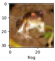
Let’s now take a closer look at the the concept of CNN using a simple demo for Image classification in Python. We will use CIFAR-10 dataset as it has 10 different categories of images naming:-

Airplane, Automobile, Bird, Cat, Deer, Dog, Frog, Horse, Ship, Truck.

The dataset has 60,000 color images (RGB) at 32px x 32px belonging to 10 different classes (6000 images/class). The dataset is divided into 50,000 training and 10,000 testing images.

Importing the Libraries

Let's start by importing the required libraries and load the dataset

#import the necessary libraries
import tensorflow as tf
from tensorflow.keras import datasets, layers, models
import matplotlib.pyplot as plt
import numpy as np

#load the dataset and check the shape of the dataset
(X_train, y_train), (X_test,y_test) = datasets.cifar10.load_data()
X_train.shape, y_train.shape, X_test.shape, y_test.shape

Next, convert the 2-D array to 1-D array,

#convert the 2-D array to 1-D array
y_train = y_train.reshape(-1,)
y_test = y_test.reshape(-1,)

define a list named 'classes' that contains the names of different categories present in the CIFAR10 dataset

#different categories present in the dataset
classes = ["airplane","automobile","bird","cat","deer","dog","frog","horse","ship","truck"]

and plot the image using a defined function.

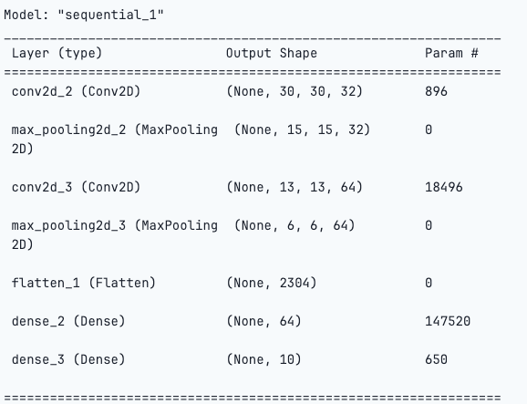
The code provided below is for building a Convolutional Neural Network (CNN) using the Keras library.

#biuld a CNN to train in the image dataset here we are using Max Pool
model = models.Sequential([
    layers.Conv2D(filters=32, kernel_size=(3, 3), activation='relu', input_shape=(32, 32, 3)),
    layers.MaxPooling2D((2, 2)),
    
    layers.Conv2D(filters=64, kernel_size=(3, 3), activation='relu'),
    layers.MaxPooling2D((2, 2)),
    
    layers.Flatten(),
    layers.Dense(64, activation='relu'),
    layers.Dense(10, activation='softmax')
])

Let us break down the code for better understanding:

1. Sequential Model:
   • The Sequential model is a linear stack of layers, allowing for the creation of the neural network layer by layer.
2. Convolutional Layers:
   • layers.Conv2D(filters=32, kernel_size=(3, 3), activation='relu', input_shape=(32, 32, 3)): This is the first convolutional layer with 32 filters, a kernel size of (3, 3), ReLU activation function, and an input shape of (32, 32, 3) indicating images with a size of 32x32 pixels and 3 color channels (RGB).
   • layers.MaxPooling2D((2, 2)): This is the first max pooling layer with a pool size of (2, 2), which reduces the dimensions of the feature maps.
   • layers.Conv2D(filters=64, kernel_size=(3, 3), activation='relu'): This is the second convolutional layer with 64 filters and a kernel size of (3, 3).
   • layers.MaxPooling2D((2, 2)): This is the second max pooling layer.
3. Flatten Layer:
   • layers.Flatten(): This layer flattens the output from the previous layer into a one-dimensional array. It prepares the data for the fully connected layers.
4. Dense (Fully Connected) Layers:
   • layers.Dense(64, activation='relu'): A fully connected layer with 64 neurons and ReLU activation.
   • layers.Dense(10, activation='softmax'): The final dense layer with 10 neurons (corresponding to the number of classes in the dataset) and a softmax activation function, which is typical for multi-class classification problems. The softmax activation normalizes the output to represent class probabilities.

This CNN architecture consists of convolutional layers for feature extraction, max pooling layers for spatial reduction, and fully connected layers for classification.

Compile the model for training by specifying the optimizer, loss function and metrics for model evaluation.

model.compile(optimizer='adam',
              loss='sparse_categorical_crossentropy',
              metrics=['accuracy'])

1. Optimizer (optimizer='adam'):
   • The optimizer is responsible for updating the weights of the neural network during training. 'adam' is a popular optimization algorithm that adapts the learning rates for each parameter individually.

Finally, fit the model using the training dataset, in this case we are using 10 epoch.

1. Loss Function (loss='sparse_categorical_crossentropy'):
   • The loss function is a measure of how well the model performs. 'sparse_categorical_crossentropy' is often used for classification problems with multiple classes. It calculates the cross-entropy loss between the predicted probabilities and the true labels. In this case, the true labels are provided as integers (e.g., 0, 1, 2) without the need for one-hot encoding.
2. Metrics (metrics=['accuracy']):
   • Metrics are used to evaluate the performance of the model. Here, 'accuracy' is specified as the metric, which calculates the proportion of correctly classified samples. This is a common metric for classification tasks.

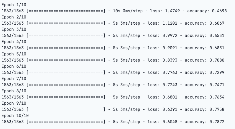
Finally, fit the model using the training dataset, in this case we are using 10 epochs.

model.fit(X_train, y_train, epochs=10)

For 10 epochs we can see the output as follows:

Once the training is successful use the test data to evaluate the model performance

As we can notice that the loss is decreasing with every epoch. This is a good sign. But it starts fluctuating at the end, which could mean the model is overfitting the training data.

model.evaluate(X_test,y_test)

313/313 [==============================] - 1s 2ms/step - loss: 0.9071 - accuracy: 0.7040

Here, the model accuracy is slightly low in the test data than the train data.

We've successfully constructed a Convolutional Neural Network using TensorFlow and Keras from the ground up!

#getting the predicted classes
y_classes = [np.argmax(pred_class) for pred_class in y_pred]

Please feel free to click the link provided to view the entire notebook.

Emerging Trends and Innovations

Pooling layers play a crucial role in Convolutional Neural Networks (CNNs). They contribute to reducing dimensionality, introducing translation invariance, and aiding in the extraction of features. Several novel approaches are emerging these days, as well. However, an ideal pooling method should be able to extract useful information and also reduce overfitting.

A recently proposed method calculates the weighted average of the dominant features known as Avg-topk. Through extensive experiments, it has been shown that the Avg-TopK pooling method consistently attains higher accuracy in image classification compared to conventional pooling methods. This approach has proven to be highly efficient to address the drawbacks caused by the max and average pooling layers in CNN.

The results from this pooling approach have proven to overcome the information loss which was a major disadvantage in traditional pooling layers.

Researchers are increasingly exploring novel pooling strategies beyond the conventional max and average pooling methods. Techniques like Inter-map Pooling, Rank-based Average Pooling, Per Pixel Pyramid Pooling, Weighted Pooling, and Genetic-based Pooling methods are gaining prominence for their efficiency and ability to capture global context.

These evolving trends in pooling reflect a continuous effort to enhance the robustness, interpretability, and generalization capabilities of CNNs across diverse applications, ranging from image classification to object detection and segmentation.

Conclusion

In this article we understood how convolution operations take place in CNN. We also understood pooling an important concept in the CNN architecture and how they work. We were also successful in building a CNN model from scratch using Keras and tensorflow framework.

In conclusion, pooling layers in Convolutional Neural Networks (CNNs) play a major role in enhancing computational efficiency, managing complexity, and extracting crucial features from input data.

While traditional max and average pooling methods remain fundamental, few of the emerging trends such as global pooling, attention mechanisms, and Avg-topk signifies a dynamic evolution in the field.

As research in this area progresses, these innovative approaches contribute significantly to the advancement of CNN architectures, leading to more robust and sophisticated models.

We hope you enjoyed the article! Thank you for reading!!

Resources

• Understanding & Interpreting Convolutional Neural Network Architectures
• Pooling Methods in Deep Neural Networks, a Review
• Introduction To Pooling Layers In CNN
• Avg-topk: A new pooling method for convolutional neural networks
• Pooling in a CNN: Pooling Layers Explained
• Keras Pooling Layers
• Pooling In Convolutional Neural Networks
• Writing CNNs from Scratch in PyTorch
• Code Reference