Nuts and Bolts of NumPy Optimization Part 1: Understanding Vectorization and Broadcasting

Libraries that speed up linear algebra calculations are a staple if you work in fields like machine learning, data science or deep learning.  NumPy, short for Numerical Python, is perhaps the most famous of the lot, and chances are you've already used it. However, merely using NumPy arrays in place of vanilla Python lists hardly does justice to the capabilities that NumPy has to offer.

In this series I will cover best practices on how to speed up your code using NumPy, how to make use of features like vectorization and broadcasting, when to ditch specialized features in favor of vanilla Python offerings, and a case study where we will use NumPy to write a fast implementation of the K-Means clustering algorithm.

As far as this part is concerned, I will be covering:

1. How to properly time your code to compare vanilla Python to optimized NumPy code.
2. Why are loops slow in Python?
3. What vectorization is, and how to vectorize your code.
4. What broadcasting is, with examples demonstrating its applications.

NOTE: While this tutorial covers NumPy, a lot of these techniques can be extended to some of the other linear algebra libraries like PyTorch and TensorFlow as well. I'd also like to point out that this post is in no way an introduction to NumPy, and assumes basic familiarity with the library.

Introduction to NumPy | Codecademy

Get acquainted with NumPy, a Python library used to store arrays of numbers, and learn basic syntax and functionality.

Codecademy

Timing your code

In order to really appreciate the speed boosts NumPy provides, we must come up with a way to measure the running time of a piece of code.

We can use Python's time module for this.

import time 

tic = time.time()

# code goes here

toc = time.time()

print("Time Elapsed: ", toc - tic)

The problem with this method is that measuring a piece of code only once does not give us a robust estimate of its running time. The code may run slower or faster for a particular iteration due to various processes in the background, for instance. It is therefore prudent to compute the average running time over many runs to get a robust estimate. To accomplish this, we use Python's timeit module.

import timeit 

setup = '''
import numpy as np 
'''

snippet = 'arr = np.arange(100)'

num_runs = 10000

time_elapsed = timeit.timeit(setup = setup, stmt = snippet, number = num_runs)

print("Time Elapsed: ", time_elapsed / num_runs)
# Output -> Time Elapsed:  5.496922000020277e-07

The timeit.timeit method has three arguments:

1. setup is a string that contains the necessary imports to run our snippet.
2. stmt is the string describing our code snippet.
3. number is the number of runs over which the experiment has to be run.

timeit can also be used to measure the run times of functions too, but only functions which don't take any arguments. For this, we can pass the function name (not the function call) to the timeit.timeit method.

import timeit 

setup = '''
import numpy as np 
'''

def fn():
    return np.arange(100)

num_runs = 10000

time_elapsed = timeit.timeit(setup = setup, stmt = fn, number = num_runs)

print("Time Elapsed: ", time_elapsed / num_runs)

If you are using an iPython console or Jupyter Notebook, you can use the %timeit magic command. The output is much more detailed than for the normal timeit.timeit call.

%timeit arr = np.arange(100)

# output -> 472 ns ± 7 ns per loop (mean ± std. dev. of 7 runs, 1000000 loops each)

A word about loops

Whenever one is looking for bottlenecks in code, especially python code, loops are a usual suspect. Compared to languages like C/C++ , Python loops are relatively slower. While there are quite a few reasons why that is the case, I want to focus on one particular reason: the dynamically typed nature of Python.

Python first goes line-by-line through the code, compiles the code into bytecode, which is then executed to run the program. Let's say the code contains a section where we loop over a list. Python is dynamically typed, which means it has no idea what type of objects are present in the list (whether it's an integer, a string or a float). In fact, this information is basically stored in every object itself, and Python can not know this in advance before actually going through the list. Therefore, at each iteration python has to perform a bunch of checks every iteration  like determining the type of variable, resolving it's scope, checking for any invalid operations etc.

Contrast this with C, where arrays are allowed to be consisting of only one data type, which the compiler knows well ahead of time. This opens up possibility of many optimizations which are not possible in Python. For this reason, we see loops in python are often much slower than in C, and nested loops is where things can really get slow.

Vectorization

OK! So loops can slow your code. So what to do now? What if we can restrict our lists to have only one data type that we can let Python know in advance? Can we then skip some of the per-iteration type checking Python does to speed up our code. NumPy does something similar. NumPy allows arrays to only have a single data type and stores the data internally in a contiguous block of memory. Taking advantage of this fact, NumPy delegates most of the operations on such arrays to optimized, pre-compiled C code under the hood.

In fact, most of the functions you call using NumPy in your python code are merely wrappers for underlying code in C where most of the heavy lifting happens. In this way, NumPy can move the execution of loops to C, which is much more efficient than Python when it comes to looping. Notice this can be only done as the array enforces the elements of the array to be of the same kind. Otherwise, it would not be possible to convert the Python data types to native C ones to be executed under the hood.

Let's take an example. Let's write a short piece of code that takes two arrays and performs element-wise multiplication. We put the code in a function just so that we can conveniently time our code later.

def multiply_lists(li_a, li_b):
    for i in range(len(li_a)):
    	li_a[i] * li_b[i]
    

Don't worry about not storing the value each iteration. The point of this exercise to merely see the performance of certain operations and not really bother about the results. We just want to see how a particular number of multiplication operations take.

However, if we were using NumPy arrays, we would not need to write a loop. We can simply do this like shown below.

arr_a = np.array(li_a)
arr_b = np.array(li_b)

def multiply_arrays(arr_a, arr_b):
	arr_a * arr_b

How does this happen? This is because internally, NumPy delegates the loop to pre-compiled, optimized C code under the hood. This process is called vectorization of the multiplication operator. Technically, the term vectorization of a function means that the function is now applied simultaneously over many values instead of a single value, which is how it looks from the python code ( Loops are nonetheless executed but in C)

Now that we have used a vectorized function in place of the loop, does it provide us with a boost in speed? We run repeat the experiment 5 times ( -r flag) , with the code being executed 10000 times ( -n flag ) over each run.

%timeit -n 10000 -r 5 multiply_lists(li_a, li_b)
%timeit -n 10000 -r 5 multiply_arrays(arr_a, arr_b)

The following is my output.

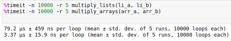
Times on your machine may differ depending upon processing power and other tasks running in background. But you will nevertheless notice considerable speedups to the tune of about 20-30x when using the NumPy's vectorized solution.

Note that I'm using the %timeit magic here because I am running the experiments in the Jupyter cell. If you are using plain python code, then you would have to use timeit.timeit function. The output of the timeit.timeit function is merely the total time which you will have to divide with number of iterations.

import timeit
total_time = timeit.timeit("multiply_lists(li_a, li_b)", "from __main__ import multiply_lists, li_a, li_b", number = 10000)

time_per_run = total_time / 10000

print(time_per_run)

Also, from now on, when I mention the phrase vectorizing a loop, what I mean is taking a loop and implementing the same functionality using one of NumPy's vectorized functions.

In addition to vectorizing a loop which performs operations on two arrays of equal size, we can also vectorize a loop which performs operations between an array and a scalar. For example, the loop:

prod = 0
for x in li_a:
	prod += x * 5

Can be vectorized as:

np.array(li_a) * 5
prod = li_a.sum()

A practical example: L2 Distance between Images

Let's now take a practical example. Something that you will encounter often if you are working with vision based Machine Learning. Let's suppose you have two images and you want to compute the L2 distance between them. This can be described by

$$ L2(I_1, I_2) =  \sum_{x} \sum_{y} \sum_{z} (I_1[x,y,z] - I_2[x,y,z])^2 $$

This simply means take a squared difference of each pixel present in the RGB image and then add these differences up. We compare the running times for a loop-based and a vectorized implementation. However notice that in our previous comparison, we used a Python list for the loop version and a NumPy array for the vectorized version. Can it be the case that it's the NumPy array, and not vectorization that makes the difference (that is, can python loops using NumPy arrays be equally fast? )

To validate that, in this example we will use NumPy array for both the loop and the vectorized version to see what really gives us the speed benefits. The loop operation requires the use of a triply nested loop, which is where things can get painfully slow. (Generally, the more deeply nested your loop is, slower would be the execution)

# Used to load images
import cv2 

# load the images
image1 = cv2.imread("image1.jpeg").astype(np.int32)
image2 = cv2.imread("image2.jpeg").astype(np.int32)


# Define the function that implements the loop version
def l2_loop(image1, image2):
    height, width, channels = image1.shape
    distance = 0
    
    for h in range(height):
        for w in range(width):
            for c in range(channels):
                distance += (image1[h][w][c] - image2[h][w][c])**2

# Define the vectorised version
def l2_vectorise(image1, image2):
    ((image1 - image2)**2).sum()

Let us now measure the time taken by our scripts over 100 runs, repeated 3 times. Running the loop based version can take a while.

%timeit -n 100 -r 3 l2_loop(image1, image2)
%timeit -n 100 -r 3 l2_vectorise(image1, image2)

We see that the vectorized version is about 2500 times faster than the loop version. Not bad!

Broadcasting

What happens if we want to vectorize a loop where we are dealing with arrays that don't have similar sizes?

Let's start with a very simple example. Suppose I have a matrix of shape (3,4) containing 3 rows and 4 columns. Now, lets say that I want to add a column vector to each of the columns in the grid. To make this clear, this is what I am trying to achieve.

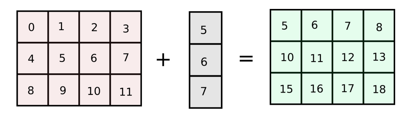
This can be accomplished in a couple of ways. We can loop over the columns of the matrix, and add each columns.

arr = np.arange(12).reshape(3,4)

col_vector = np.array([5,6,7])

num_cols = arr.shape[1]

for col in range(num_cols):
	arr[:, col] += col_vector

    
	

However, if the number of columns in our original array arr are increased to a very large number, the code described above will run slow as we are looping over the number of columns in Python. How about making a matrix of equal size as the original array with identical columns ? (We will refer this approach as column-stacking approach)

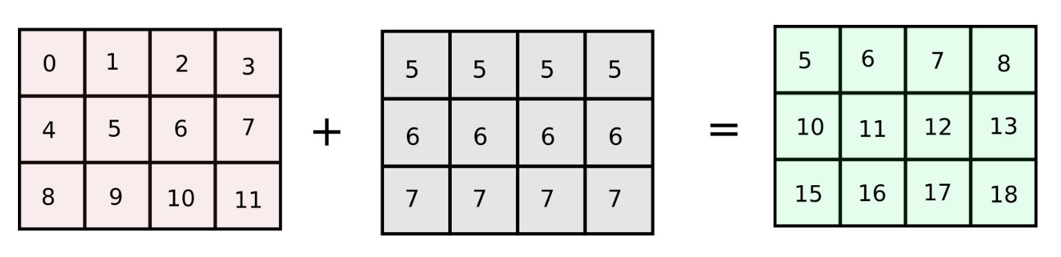
arr = np.arange(12).reshape(3,4)
add_matrix = np.array([col_vector,] * num_cols).T

arr += add_matrix

This gives us a much faster solution. While this approach worked well in case of a 2-dimensional array, applying the same approach with higher dimensional arrays can be a bit tricky.

The good news, however, is that NumPy provides us with a feature called Broadcasting, which defines how arithmetic operations are to be performed on arrays of unequal size. According to the SciPy docs page on broadcasting,

Subject to certain constraints, the smaller array is “broadcast” across the larger array so that they have compatible shapes. Broadcasting provides a means of vectorizing array operations so that looping occurs in C instead of Python

Under the hood, NumPy does something similar to our column-stacking approach. However, we don't have to worry about stacking arrays in multiple directions explicitly.

Let us now understand the rules of Broadcasting in NumPy. These are the certain constraints that the definition above talks about. Two arrays must fulfill these conditions for the smaller of them to be broadcasted over the larger one.

Rules of Broadcasting

Before we begin, one important definition we need to know is the rank of the array  in NumPy. The rank is the total number of dimensions a NumPy array has. For example, an array of shape (3, 4) has a rank of 2 and array of shape (3, 4, 3) has a rank of 3. Now onto the rules.

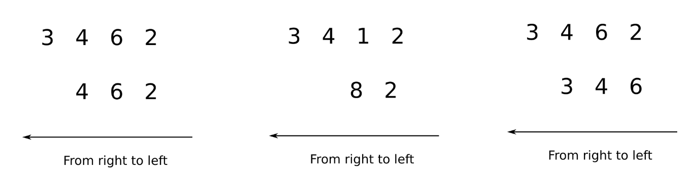
1. To deem which two arrays are suitable for operations, NumPy compares the shape of the two arrays dimension-by-dimension starting from the trailing dimensions of the arrays working it's way forward.  (from right to left)
2. Two dimensions are said to be compatible if both of them are equal, or either one of them is 1.
3. If both the dimensions are unequal and neither of them is 1, then NumPy will throw an error and halt.

Arrays with Equal Ranks

We first consider the case where the ranks of the two arrays we are dealing with are the same. The following image demonstrates which set of arrays are compatible and which aren't.

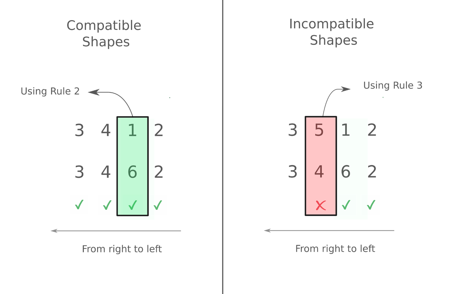
As you can see, we work from left to right.  In case of the second example on the right, we start working from left, but when we arrive at the 2nd dimension (4 and 5 for both arrays resp.), we see there's a difference and neither of them is 1. Therefore, trying to do an operation with them leads to an error

arr_a = np.random.rand(3,4,6,2) # random array of shape (3,4,6,2)
arr_b = np.random.rand(3, 5, 1, 2)

arr_a + arr_b   # op throws an error 

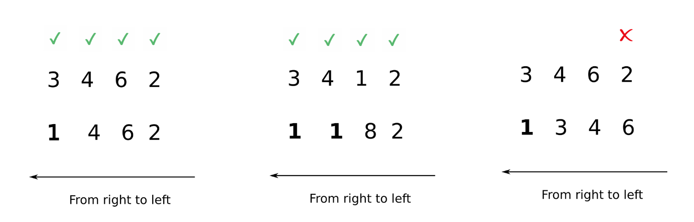
In the first example on the left, we encounter different dimensions in the 3rd dimension ( 1 and 6 for both arrays respectively). However, according to rule 2, these dimensions are compatible. Every other dimension is the same. So we can perform arithmetic operation with the two arrays.

arr_a = np.random.rand(3,4,6,2) # random array of shape (3,4,6,2)
arr_b = np.random.rand(3, 4, 1, 2) 

arr_a + arr_b   # op goes through without throwing an error. 

Arrays with Unequal Ranks

Arrays having unequal ranks can be operated upon as well subject to certain conditions. Again, we apply the rule of moving from left to right and comparing the two arrays. Let's consider the following examples.

In the image above, we see in the first case, the first array has the rank of 4 while the second array is the rank of 3. We can  compare from left to right for 3 dimensions, after which the second array has no dimensions. In order to compare two such arrays, Numpy appends forward dimensions of size 1 to the smaller array so that it has a rank equal to the larger array. So all the comparisons above can be treated as.

Now, comparisons can be easily made.  

Note that I use italics for appending because this is just a way to visualize what NumPy is doing. Internally, there is no appending.

What happens during Broadcasting

While it's easy to understand how an operation is performed when both the dimensions are similar, let's now understand how an operation is performed when one of the dimensions is 1 (Rule 2).

For this consider our example from above where we wanted to add a column vector to all columns of a matrix. The shapes of the arrays are (3,4) and (3,), which cannot be added according to rules of broadcasting. However, if we shape the column vector of shape (3,) to (3, 1), the two shapes become compatible.

col_vector = col_vector.reshape((3, 1)) # reshape the array
arr += col_vector                      # addition goes through!

But wait, what exactly happened? How did the second dimensions, 4 and 1 for arr and col_vector respectively reconcile?

In such cases, NumPy will perform the operation as if the second array, of size (3, 1) was an array of shape (3,4). The values in the dimension having size 1  (In this case the second dimension of the original array was of shape (3, 1)) will be repeated across 4 dimensions now to create an array of shape (3, 4).  To understand this, consider the second array, and the value of it's second dimension.

print(col_vector[0, :])       # output -> [5]
print(col_vector[1, :])       # output -> [6]
print(col_vector[2, :])       # output -> [7]

Now, the newly created array, of the shape (3, 4) will have the repeated values in it's second dimension. To aid our imagination, we use the function np.brodcast_to which gives us an idea of how the new broadcasted array is created.

broadcasted_col_vector = np.broadcast_to(col_vector, (3,4))


print(broadcasted_col_vector[0,:])   # output -> [5, 5, 5, 5]
print(broadcasted_col_vector[1,:])   # output -> [6, 6, 6, 6]
print(broadcasted_col_vector[2,:])   # output -> [7, 7, 7, 7]

As you can see, the values in the second dimension (which original had size 1),has been repeated 4 times to create a dimension of size 4.

To pictorially represent what's going on, the array is repeated across it's second dimension 4 times to create an equal array.

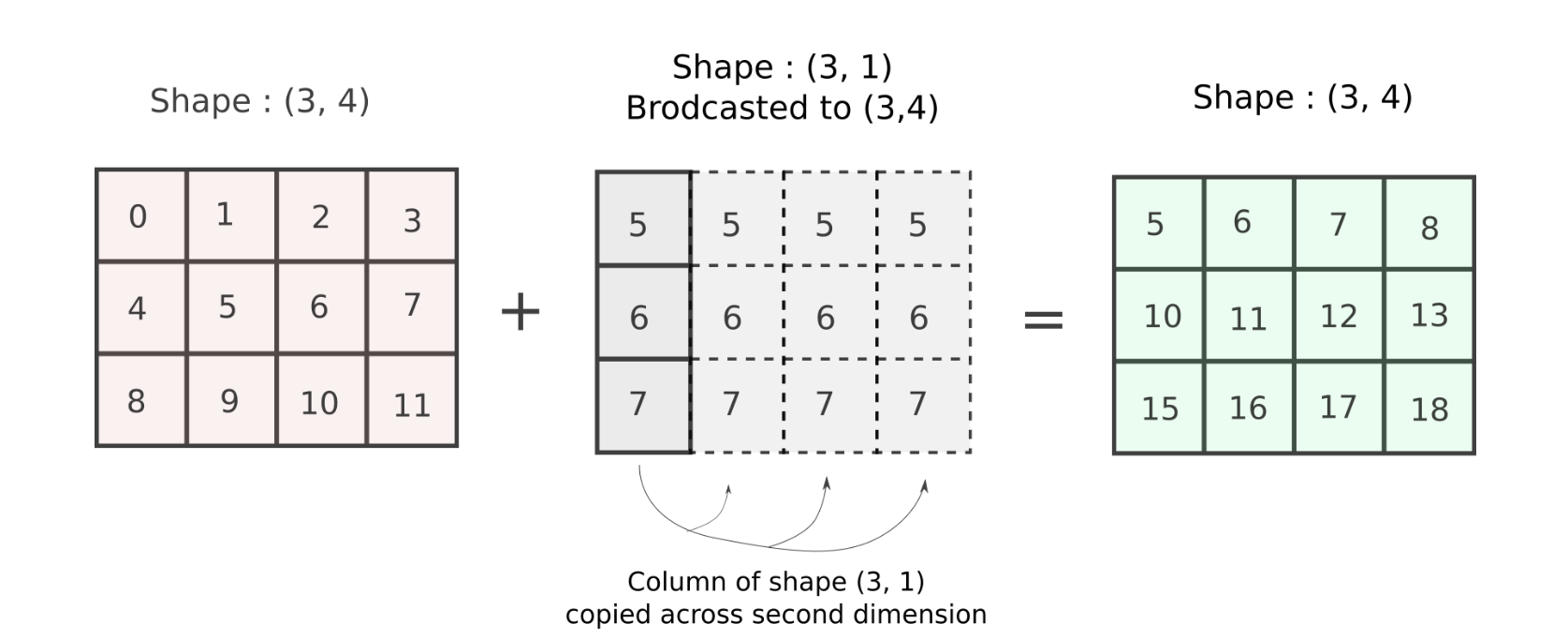
This is exactly what we did with our column-stack operation! The result of the addition is what we wanted!

Let's consider the case for a 3-D array of shapes (3, 4, 5) and (1, 4, 5)

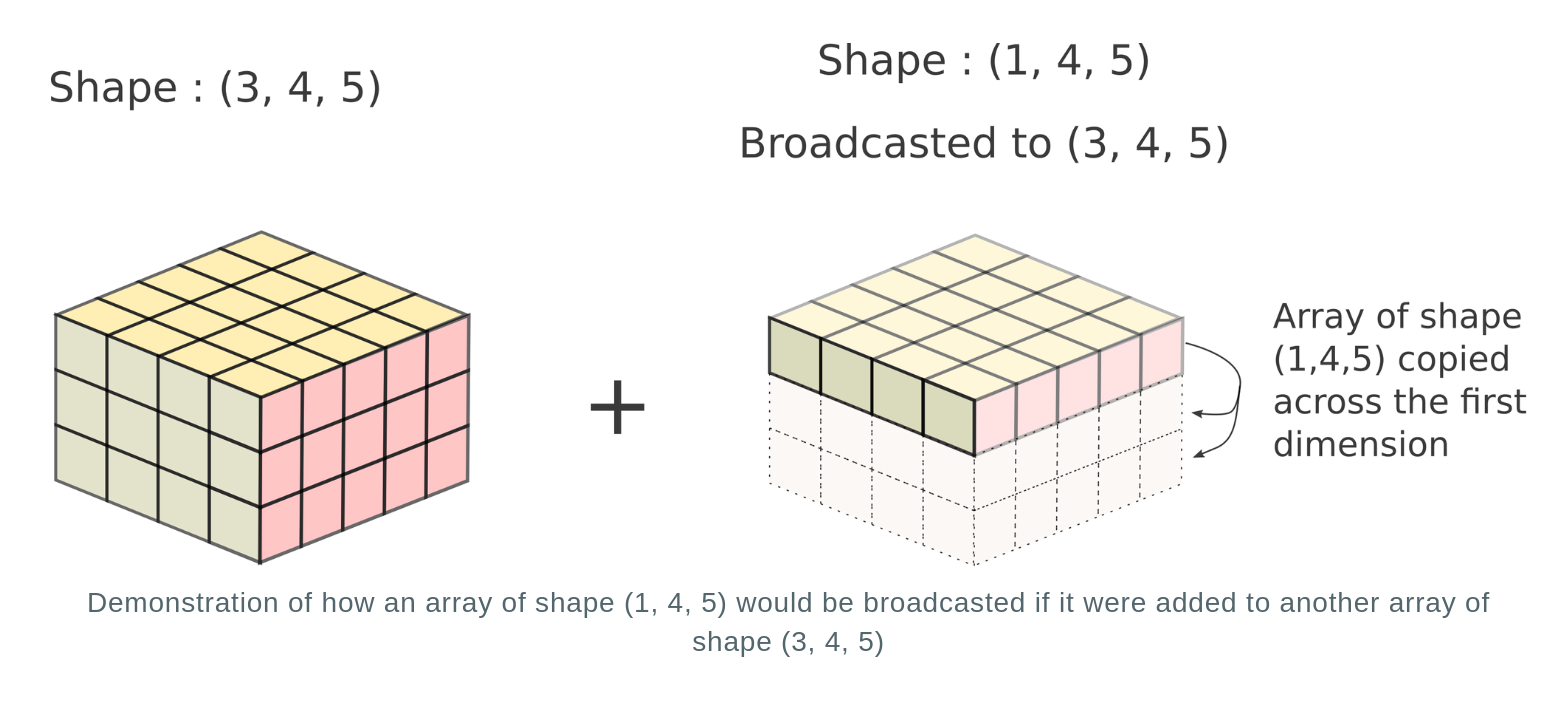
In reality, no new array is actually created. The repeated array is merely a mental tool to image how the operation would be performed. Instead, the computation is repeated across multiple dimensions without creation of a new array. This is akin to broadcasting values of the dimension of the first array having size 1 across multiple positions to the values in the dimension  of the second array having size of more than 1. Hence, this process is termed as broadcasting.

A practical example: Adding color to an Image

Let's suppose you have an image, and for each pixel, you want to increase red values by 10,  green values by 5 and blue values by 15.

This can be easily accomplished by broadcasting.  An image is represented as a matrix having a shape (H, W, C) if we read it in using OpenCV. Let's read an image!

img = cv2.imread("image1.jpeg")
print(img.shape)

# output -> (768, 1024, 3)

Now, the channels are encoded in the third dimension of this array. We want to add 10, 5, 15  to the first channel described by img[ : , : ,0], second channel described by img[ : , : ,1], and third channel described by img[ : , : ,2] respectively. This can be easily done using the following piece of code.

add_color = [10, 5, 15]
img += add_color

The shape of our image is (768, 1024, 3) whereas our color vector has shape (3,). On addition, this array will be resized to  (1, 1, 3) and subsequently, each color value will be broadcasted across the the R, G, B channels respectively.

However, some applications of deep learning require the image to be stored in format [C, H, W. In that case our image would have the shape (3, 768, 1024). In order to to do the same operation, we will have to reshape our color vector to shape  (3, 1, 1) so that it's compatible. Then, we can easily add the two.

img = img.transpose((2, 0, 1))           # change shape to (3, 768, 1024)
add_color = add_color.reshape((3,1,1,))
img += add_color

Visualizing Loops as Arrays

One thing that has always aided me when it comes to vectorization and broadcasting is to visualize whatever goes on in a loop as an operation being performed on an array

Suppose, we have two arrays of unequal size. We want to take a product of every combination of elements of the two arrays and then sum them up. For example, for arrays [1, 2, 3] and [4, 5] , the sum would be

$$ 1*4 + 2 * 4 + 3 * 4 + 1*5 + 2*5 + 3 * 5 $$

Using loops, that is how we do it,

sum  = 0

arr1 = np.array([1, 2, 3])
arr2 = np.array([4, 5])

for i in arr1:
	for j in arr2:
    	sum += i*j

Simply enough right? But this is a nested loop, and if the sizes of these arrays becomes too large, then the running times will be increase too.

How do we get rid of these two loops and come up with a vectorized solution instead. For this, pay attention to what the loop variables i and j are doing. i goes from 1 to 3 while j goes from 4 to 5. In the loop, we have every possible combination of [i,j] which we multiply and then sum.

Can we have a array, a 2-D one, whose indices [i,j] represent product of every such combination? If yes, we can have a NumPy array to represent this array and we can do away with loops and simply sum the elements of the array!  This is how the array would look like.

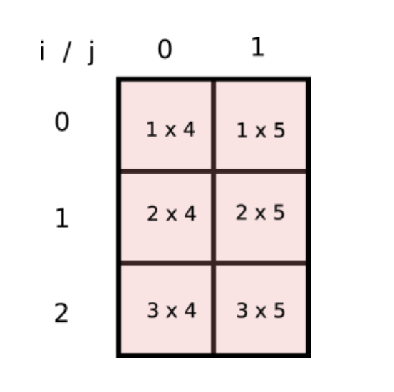
This is nothing but the product of two arrays..

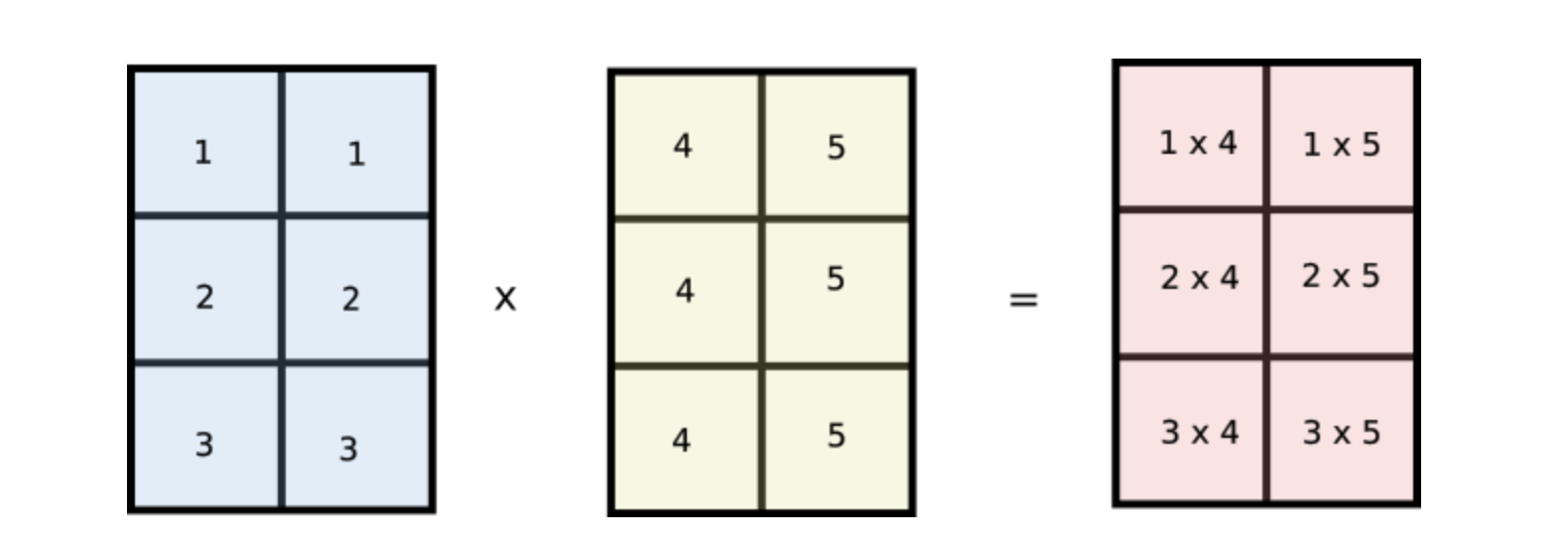
But wait, notice how values of i are repeated across columns of the first array and values of j are repeated across rows of the second array. Does this look familiar? Notice if we reshape our original arr1 and arr2 arrays to [3,1] and [1,2] respectively and multiply the two arrays, then they would be broadcasted like the following.

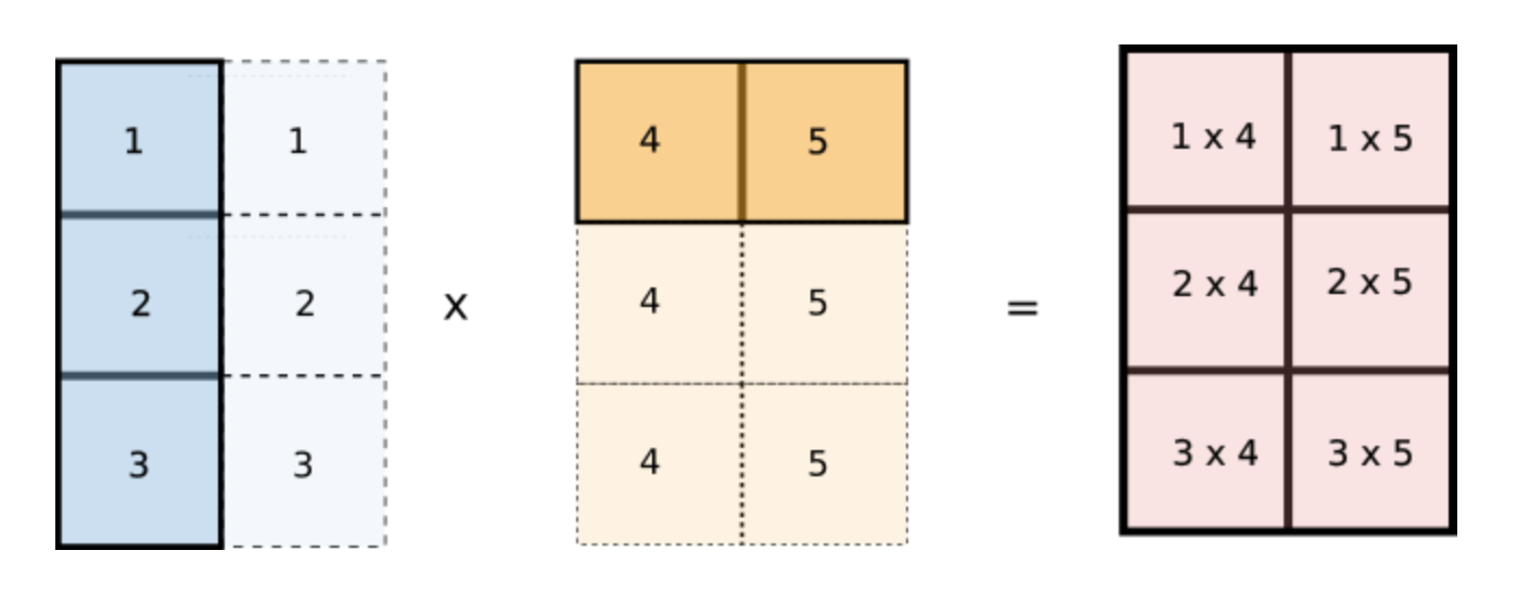
This is exactly what we want! We can now implement this in code.

arr1 = arr1[:, None]    # reshape to (3, 1)
arr2 = arr2[None, :]    # reshape to (1, 2)
 
sum = (arr1 * arr2).sum()

Conclusion

Phew! That was one detailed post! Truth be said, vectorization and broadcasting are two cornerstones of writing efficient code in NumPy and that is why I thought the topics warranted such a long discussion. I encourage you to come up with toy examples to get a better grasp of the concepts.

In the next part, we will use the things we covered in this post to optimize a naive implementation of the K-Means clustering algorithm (implemented using Python lists and loops) using vectorization and broadcasting, achieving speed-ups of 70x!

Until then, Happy Coding!