Gradient Descent and Optimization In Deep Learning

The most common method underlying many of the deep learning model training pipelines is gradient descent. But vanilla gradient descent can encounter several problems, like getting stuck at local minima or the problems of exploding and vanishing gradients. To fix these problems several variants of the gradient descent have been devised over time. We will take a look at the most common ones in this article, and benchmark them for some optimization problems.

You can follow along with the code in this tutorial and run it for free from the ML Showcase.

Gradient Descent

Before we dive into optimizers, let's first take a look at gradient descent. Gradient descent is an optimization algorithm that iteratively reduces a loss function by moving in the direction opposite to that of steepest ascent. The direction of the steepest ascent on any curve, given the initial point, is determined by calculating the gradient at that point. The direction opposite to it would lead us to a minimum fastest.

Mathematically, it is a way to minimize the objective function J(𝜃), where 𝜃 represents the model’s parameters. Deep architectures make predictions by following a feed-forward mechanism in which each layer takes the output of the previous layer as input, and uses the parameters represented by 𝜃 (or as many familiar with optimization in neural networks would call them, the weights and biases), and finally outputs the transformed features that are passed onto the next layer. The output of the final layer is compared with the real output we expect, and a loss function is calculated. These parameters are then updated using backpropagation, which uses gradient descent to find the exact way in which the parameters ought to be updated. These updates to the parameters are dependent on the gradient and the learning rate of the optimization algorithm.

The parameter updates based on gradient descent follow the rule:

θ = θ − η ⋅ ∇ θ J(θ)

Where η is the learning rate.

The mathematical formulation for the gradient of a 1D function with respect to its input looks like this:

While this is accurate for continuous functions, while computing gradients for neural networks we will mostly be dealing with discrete functions and calculating limits is not as straightforward as shown above.

The above mentioned method (forward differencing) turns out to be less accurate, since the truncation error is of the order O(h). Instead a central differencing scheme is used, that looks like this:

In the central differencing method, the truncation error is of the order O(h2). The truncation error is based on the Taylor expansions of the two formulations. A good explanation thereof can be found here and here.

Gradient Descent Variants

Gradient descent is preferred over other iterative optimization methods, like the Newton Rhapson method, since Newton’s method uses first and second order derivatives at each time-step, making it inefficient for operating at scale.

There are several flavors of gradient descent that try to solve certain limitations of the vanilla algorithm, like stochastic gradient descent and mini-batch gradient descent that allow for online learning. While vanilla gradient descent calculates the gradient on the entire dataset, batch gradient descent allows us to update gradients while processing several batches of data, making it memory efficient when dealing with large datasets.

Vanilla Gradient Descent

Let's start by looking at how to implement vanilla and momentum gradient descent from scratch to see how the algorithm works. Then we'll visualize gradient updates for 2D functions on contour plots to get a better understanding of the algorithms.

The updates will not be based on a loss function, but simply a step in the direction opposite from the steepest ascent. To get the direction of steepest ascent, we will first write the function to calculate the gradient of a function given the point at which the gradient needs to be calculated. We also need another parameter which will define the size of our numerical differentiation steps, denoted by h.

The central differencing scheme for numerical differentiation for a function that takes multiple coordinates as input can be implemented as follows.

import numpy as np

def gradient(f, X, h):
    grad = []
    for i in range(len(X)):
        Xgplus = np.array([x if not i == j else x + h for j, x in enumerate(X)])
        Xgminus = np.array([x if not i == j else x - h for j, x in enumerate(X)])
        grad.append(f(*Xgplus) - f(*Xgminus) / (2 * h))
    return np.array(grad)

A vanilla gradient descent update will look like this:

def vanilla_update(epoch, X, f, lr, h):
    grad = gradient(f, X, h)
    X1 = np.zeros_like(X)
    for i in range(len(X)):
        X1[i] = X[i] - lr * grad[i]
    print('epoch: ', epoch, 'point: ', X1, 'gradient: ', grad)
    return X1

You can think of the learning rate as the step size for our gradient update.

We will test our algorithm on Ackley’s function, one of the popular functions for testing optimization algorithms. Ackley's function looks something like this.

import numpy as np

def ackleys_function(x, y):
    return - 20 * np.exp(- 0.2 * np.sqrt(0.5 * (x ** 2 + y ** 2))) \
           - np.exp(0.5 * (np.cos(2 * np.pi * x) + np.cos(2 * np.pi * y))) \
           + np.e + 20

Now, to finally test out our vanilla gradient descent:

if __name__ == '__main__':
    h = 1e-3
    f = ackleys_function
    point = np.array([-2., -2.])
    i = 0
    lr = 0.00001
    while True:
        new_point = vanilla_update(i+1, point, f, lr, h)
        plt.plot(*point, 'ro', ms=1)
        if np.sum(abs(new_point - point)) < h:
            print('Converged.')
            break
        point = new_point
        i += 1

The convergence criteria we use is simple. If the absolute value of the coordinates of the point do not change significantly, as determined by the value of h, we stop the algorithm.

Momentum Gradient Descent

For steep slopes, momentum gradient descent helps us accelerate down the slope faster than vanilla gradient descent. This is achieved by using a momentum term. You can think of it as adjusting the velocity of how the gradient steps are taken according to the magnitude and direction of the gradients. The momentum factor in the gradient update is a moving average of gradients until the last time step, multiplied by a constant less than 1 which guarantees the entire velocity term to converge for extremely high slopes. This helps us avoid extreme jumps while updating parameters.

To implement momentum updates, besides calculating the gradient at the current point, the gradients of previous steps have to be stored for the calculation of the momentum step. The parameter m is defined as momentum, and the function can be implemented as follows.

def momentum_update(epoch, X, f, lr, m, h, vel=[]):
    grad = gradient(f, X, h)
    X1 = np.zeros_like(X)
    for i in range(len(X)):
        vel[i] = m * vel[i] + lr * grad[i]
        X1[i] = X[i] - vel[i]
    print('epoch: ', epoch, 'point: ', X1, 'gradient: ', grad, 'velocity: ', vel)
    return X1, vel

The final loop will look like this:

if __name__ == '__main__':
    h = 1e-3
    f = ackleys_function
    point = np.array([-2., -2.])
    vel = np.zeros_like(point)
    i = 0
    lr = 0.00001
    m = 0.9
    grads = []
    while True:
        new_point, vel = momentum_update(i+1, point, f, lr, m, h, vel=vel)
        plt.plot(*point, 'bo', ms=1)
        if np.sum(abs(new_point - point)) < h:
            print('Converged.')
            break
        point = new_point
        i += 1

Gradient Descent Visualization

Getting the plots for the function in 3D:

from matplotlib import pyplot as plt
from mpl_toolkits import mplot3d

def get_scatter_plot(X, Y, function):
    Z = function(X, Y)
    fig = plt.figure()
    cm = plt.cm.get_cmap('viridis')
    plt.scatter(X, Y, c=Z, cmap=cm)
    plt.show()
    return fig


def get_contours(X, Y, function):
    Z = function(X, Y)
    fig = plt.figure()
    contours = plt.contour(X, Y, Z, colors='black',
                           linestyles='dashed',
                           linewidths=1)
    plt.clabel(contours, inline=1, fontsize=10)
    plt.contourf(X, Y, Z)
    plt.xlabel('X')
    plt.ylabel('Y')
    plt.show()
    return fig


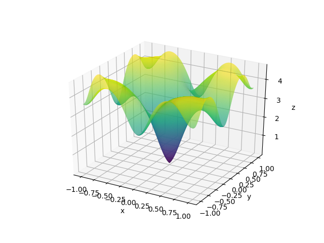
def get_3d_contours(X, Y, function):
    Z = function(X, Y)
    fig = plt.figure()
    ax = plt.axes(projection='3d')
    cm = plt.cm.get_cmap('viridis')
    ax.contour3D(X, Y, Z, 100, cmap=cm)
    ax.set_xlabel('x')
    ax.set_ylabel('y')
    ax.set_zlabel('z')
    plt.show()
    return fig
    
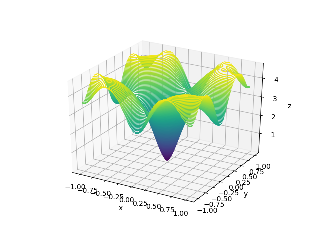
def get_surface_plot(X, Y, function):
    Z = function(X, Y)
    fig = plt.figure()
    ax = plt.axes(projection='3d')
    cm = plt.cm.get_cmap('viridis')
    ax.plot_surface(X, Y, Z, rstride=1,
                    cstride=1, cmap=cm)
    ax.set_xlabel('x')
    ax.set_ylabel('y')
    ax.set_zlabel('z')
    plt.show()
    return fig


if __name__ == '__main__':
    x = np.linspace(-1, 1, 1000)
    X, Y = np.meshgrid(x, x)
    get_scatter_plot(X, Y, ackleys_function)
    get_contours(X, Y, ackleys_function)
    get_3d_contours(X, Y, ackleys_function)
    get_surface_plot(X, Y, ackleys_function)

The visualizations look something like this.

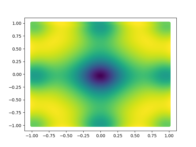
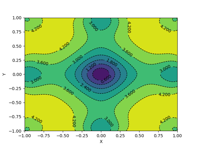
Here, X and Y happen to be a meshgrid instead of 1D arrays. We can create a meshgrid using the numpy function np.meshgrid.

You can also utilize the amazing VisPy library to create 3D visualizations fast, and study them in real time.

import sys
from vispy import app, scene


def get_vispy_surface_plot(x, y, function):
    canvas = scene.SceneCanvas(keys='interactive', bgcolor='w')
    view = canvas.central_widget.add_view()
    view.camera = scene.TurntableCamera(up='z', fov=60)
    X, Y = np.meshgrid(x, y)
    Z = function(X, Y)
    p1 = scene.visuals.SurfacePlot(x=x, y=y, z=Z, color=(0.3, 0.3, 1, 1))
    view.add(p1)
    scene.Axis(font_size=16, axis_color='r',
                     tick_color='r', text_color='r',
                     parent=view.scene)
    scene.Axis(font_size=16, axis_color='g',
                     tick_color='g', text_color='g',
                     parent=view.scene)
    scene.visuals.XYZAxis(parent=view.scene)
    canvas.show()
    if sys.flags.interactive == 0:
        app.run()
    return scene, app

This should give you a canvas to play around with the plot.

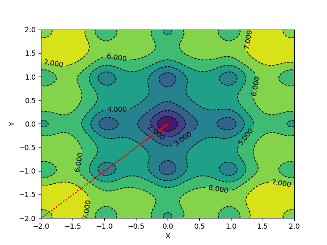
To visualize gradient descent updates on contour plots for vanilla gradient descent, use the following code.

if __name__ == '__main__':

    x = np.linspace(-2, 2, 1000)

    h = 1e-3

    f = ackleys_function

    a, b = np.meshgrid(x, x)
    Z = f(a, b)
    contours = plt.contour(a, b, Z, colors='black',
                           linestyles='dashed',
                           linewidths=1)
    plt.clabel(contours, inline=1, fontsize=10)
    plt.contourf(a, b, Z)
    plt.xlabel('X')
    plt.ylabel('Y')

    point = np.array([-2., -2.])

    i = 0
    lr = 0.00001
    while True:
        new_point = vanilla_update(i+1, point, f, lr, h)
        plt.plot(*point, 'ro', ms=1)
        if np.sum(abs(new_point - point)) < h:
            print('Converged.')
            break
        point = new_point
        i += 1

    plt.show()

The algorithm takes 139 epochs to converge, and the gradient updates look something like this:

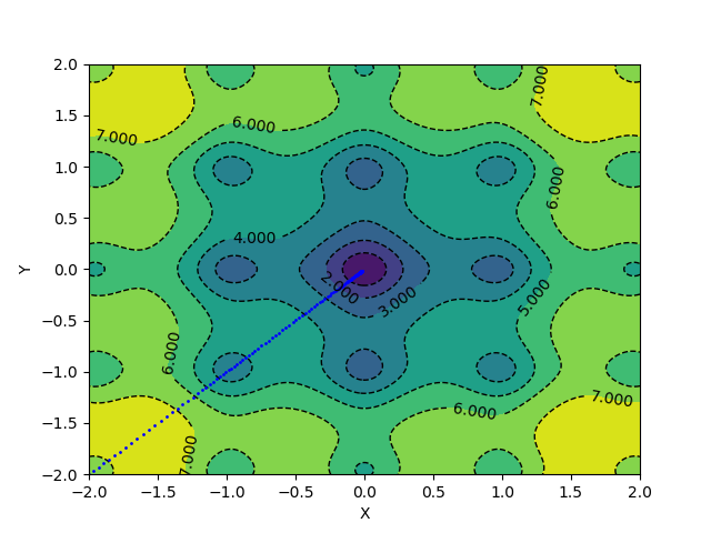
For applying momentum updates and plotting, you can use the following code:

if __name__ == '__main__':

    x = np.linspace(-2, 2, 1000)

    h = 1e-3

    f = ackleys_function

    a, b = np.meshgrid(x, x)
    Z = f(a, b)
    contours = plt.contour(a, b, Z, colors='black',
                           linestyles='dashed',
                           linewidths=1)
    plt.clabel(contours, inline=1, fontsize=10)
    plt.contourf(a, b, Z)
    plt.xlabel('X')
    plt.ylabel('Y')
    
    point = np.array([-2., -2.])
    vel = np.zeros_like(point)

    i = 0
    lr = 0.00001
    m = 0.1
    grads = []
    while True:
        new_point, vel = momentum_update(i+1, point, f, lr, m, h, vel=vel)
        plt.plot(*point, 'bo', ms=1)
        if np.sum(abs(new_point - point)) < h:
            print('Converged.')
            break
        point = new_point
        i += 1
    plt.show()

With the same learning rate and a momentum of 0.1, the above update scheme converges in 127 epochs.

Popular Gradient Descent Implementations

There are several implementations of the gradient descent algorithm, and all of them have small tweaks meant to solve a particular issue.

Some of the popular gradient descent algorithms include:

1. Nesterov Momentum - As we discussed, in momentum-based gradient descent the velocity term consists of a moving average until the previous time step. In Nesterov momentum, the current time step is considered, giving the algorithm a sort of predictive capacity for how to adjust updates for the next time step. The gradient of the next step is calculated by finding an approximate position after the next update by taking the momentum into account.
2. Adam - Adaptive Moment Estimation, also known as Adam optimizer, computes adaptive learning rates for each optimization step by looking at first and second moments calculated from gradients and a constant parameter. Part of it is similar to momentum, but Adam performs better in cases where the velocity for momentum-based optimization is high, as it provides an opposing force for gradient steps in terms of the second moment. The algorithm uses a de-biasing mechanism to make sure it doesn't always converge to trivial values.
3. AdaGrad - Adagrad calculates the adaptive learning rate by assigning higher weights to infrequently occurring features, as compared to the ones that occur frequently. It accumulates squared gradients in the same way momentum accumulates gradients. This makes the optimizer perform better on sparse data. Adagrad was used to train the GloVe word vectors.
4. AdaMax - The Adam algorithm can be modified to scale the second moment according to the L2 norm values, instead of using the original values. But then the parameter is in turn squared as well. Instead of using squared terms, one could use any exponent n. While for larger values such a gradient update tends to be unstable, if the parameter n tends to infinity, it provides us with a stable solution. The velocity term obtained according to this regularization of gradients is then used to update the weights of the model.
5. AdamW - AdamW optimizer is in essence Adam that uses L2 regularization of weights. The common implementation for L2 regularization modifies the gradient values with the decayed weights, whereas in the AdamW implementation, the regularization is done during the gradient update step. This mild change seems to change the results in a significant manner.
6. AdaDelta - Like Adagrad, Adadelta uses accumulated squared gradients but only in a set window of steps. The gradients aren't stored, but are dynamically calculated. So on every step, the memory utilization is optimized due to the dependence only on the previous average and the current gradient.  

A great resource to learn about the popular gradient descent algorithms in more mathematical detail can be found here. Implementations of some of these can be found here.

Benchmarking Optimizers

Lets see how some of these optimizers perform against each other. We will be using the CIFAR10 dataset for the benchmarking. You can also follow along with the code from the ML Showcase, and run it for free on Gradient.

Let's import all the things we need to get started with our training script. We will be using PyTorch optimizers and their ResNet18 implementation. We will use Matplotlib to visualize our results.

import torch
from torch import nn
from torch import optim
from torch.utils.data import RandomSampler, DataLoader

from torchvision import models
from torchvision import transforms
from torchvision.datasets import CIFAR10 as cifar
from torchvision import datasets

import time
import pickle
import random
import numpy as np
from tqdm import tqdm
from matplotlib import pyplot as plt

To make sure our results are reproducible, lets set the PRNG seeds for torch, NumPy, and the Python random module.

We then create an augmented and normalized dataset. The CIFAR dataset is used to create our train and test dataloaders.

torch.manual_seed(0)
torch.cuda.manual_seed(0)
np.random.seed(0)
random.seed(0)

DATA_PATH = 'cifar'

trans = transforms.Compose([            [
                transforms.RandomHorizontalFlip(),
                transforms.RandomCrop(32, padding=4),
                transforms.ToTensor(),
                transforms.Normalize(
                    mean=[n/255. for n in [129.3, 124.1, 112.4]], 
                    std=[n/255. for n in [68.2,  65.4,  70.4]]
                )
        ])


train = cifar(DATA_PATH, train=True, transform=trans, download=False)
test = cifar(DATA_PATH, train=False, transform=trans, download=False)


batch_size = 64
train_size = len(train)
test_size = len(test)

train_dataloader = DataLoader(train, shuffle=True, batch_size=batch_size)
test_dataloader = DataLoader(test, shuffle=False, batch_size=batch_size)

We will be training a ResNet18 model for this task. The ResNet18 model by default outputs 1000 features. To make it work for our dataset, we add a linear layer with 1000 input features and 10 output features.

class Cifar10_Resnet18(nn.Module):

    def __init__(self,):
        super(Cifar10_Resnet18, self).__init__()
        self.base = models.resnet18(pretrained=True)
        self.classification = nn.Linear(in_features=1000, out_features=10)

        
    def forward(self, inputs):
        out = self.base(inputs)
        out = self.classification(out)
        return out

If using a GPU, set the device to type CUDA.

device = torch.device(type='cuda')

Lets define a dictionary of all the optimizers we'll be benchmarking so that we can create a loop to iterate through all of them. The values of the dictionary are the commands to define the optimizer put into strings. We will use the eval function to bring the optimizers to life later.

optimizers = {
        'SGD': 'optim.SGD(model.parameters(), lr=0.01, momentum=0.9)',
        'Adam': 'optim.Adam(model.parameters())',
        'Adadelta': 'optim.Adadelta(model.parameters())',
        'Adagrad': 'optim.Adagrad(model.parameters())',
        'AdamW': 'optim.AdamW(model.parameters())',
        'Adamax': 'optim.Adamax(model.parameters())',
        'ASGD': 'optim.ASGD(model.parameters())',
    }

The main training loop trains each optimizer for 50 epochs and notifies us about the training accuracy, validation accuracy, training loss, and testing loss. We use CrossEntropyLoss as our loss criterion, and finally we save all the metrics as pickle files. For every optimizer, a new model is initalized after which we use the eval function to define the optimizer according to untrained model parameters.

epochs = 50

optim_keys = list(optimizers.keys())

train_losses = []
train_accuracies = []
test_losses = []
test_accuracies = []

for i, optim_key in enumerate(optim_keys):
    print('-------------------------------------------------------')
    print('Optimizer:', optim_key)
    print('-------------------------------------------------------')
    print("{:<8} {:<25} {:<25} {:<25} {:<25} {:<25}".format('Epoch', 'Train Acc', 'Train Loss', 'Val Acc', 'Val Loss', 'Train Time'))
    
    model = Cifar10_Resnet18()
    model.to(device)

    optimizer = eval(optimizers[optim_key])
    criterion = nn.CrossEntropyLoss()
    
    model.train()
    
    optim_train_acc = []
    optim_test_acc = []
    optim_train_loss = []
    optim_test_loss = []

    for epoch in range(epochs):

        start = time.time()

        epoch_loss = []
        epoch_accuracy = []
        
        for step, batch in enumerate(train_dataloader):
            
            optimizer.zero_grad()
            
            batch = tuple(t.to(device) for t in batch)
            images, labels = batch
            
            out = model(images)
            
            loss = criterion(out, labels)
            
            confidence, predictions = out.max(dim=1)
            truth_values = predictions == labels
            acc = truth_values.sum().float().detach().cpu().numpy() / truth_values.shape[0]
            
            epoch_accuracy.append(acc)
            epoch_loss.append(loss.float().detach().cpu().numpy().mean())
            
            loss.backward()
            optimizer.step()
        
        optim_train_loss.append(np.mean(epoch_loss))
        optim_train_acc.append(np.mean(epoch_accuracy))
        
        test_epoch_loss = []
        test_epoch_accuracy = []
        
        end = time.time()
        
        model.eval()
        for step, batch in enumerate(test_dataloader):
            
            batch = tuple(t.to(device) for t in batch)
            images, labels = batch
            
            out = model(images)
            
            loss = criterion(out, labels)
            
            confidence, predictions = out.max(dim=1)
            truth_values = predictions == labels
            acc = truth_values.sum().float().detach().cpu().numpy() / truth_values.shape[0]
            
            test_epoch_accuracy.append(acc)
            test_epoch_loss.append(loss.float().detach().cpu().numpy().mean())
        
        optim_test_loss.append(np.mean(test_epoch_loss))
        optim_test_acc.append(np.mean(test_epoch_accuracy))
        
        print("{:<8} {:<25} {:<25} {:<25} {:<25} {:<25}".format(epoch+1, 
                                                                np.mean(epoch_accuracy), 
                                                                np.mean(epoch_loss), 
                                                                np.mean(test_epoch_accuracy), 
                                                                np.mean(test_epoch_loss), 
                                                                end-start))
    
    train_losses.append(optim_train_loss)
    test_losses.append(optim_test_loss)
    train_accuracies.append(optim_train_acc)
    test_accuracies.append(optim_train_acc)
    
train_accuracies = dict(zip(optim_keys, train_accuracies))
test_accuracies = dict(zip(optim_keys, test_accuracies))
train_losses = dict(zip(optim_keys, train_losses))
test_losses = dict(zip(optim_keys, test_losses))

with open('train_accuracies', 'wb') as f:
    pickle.dump(train_accuracies, f)
with open('train_losses', 'wb') as f:
    pickle.dump(train_losses, f)
with open('test_accuracies', 'wb') as f:
    pickle.dump(test_accuracies, f)
with open('test_losses', 'wb') as f:
    pickle.dump(test_losses, f)

We can plot our results using the following code.

x = np.arange(epochs) + 1

for optim_key in optim_keys:
    plt.plot(x, train_accuracies[optim_key], label=optim_key)

plt.title('Training Accuracies')
plt.legend()
plt.show()


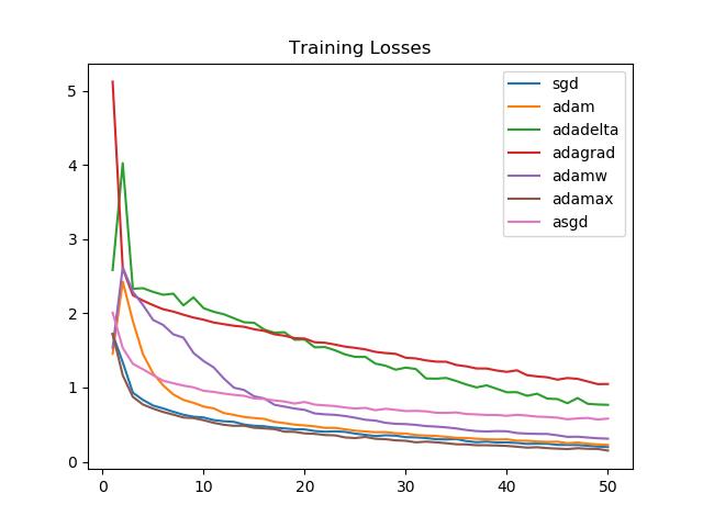
for optim_key in optim_keys:
    plt.plot(x, train_losses[optim_key], label=optim_key)

plt.title('Training Losses')
plt.legend()
plt.show()


for optim_key in optim_keys:
    plt.plot(x, test_accuracies[optim_key], label=optim_key)

plt.title('Testing Accuracies')
plt.legend()
plt.show()


for optim_key in optim_keys:
    plt.plot(x, test_losses[optim_key], label=optim_key)

plt.title('Testing Losses')
plt.legend()
plt.show()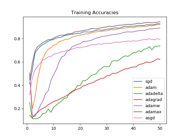

We see that Adamax, for the task we picked, consistently performs better than all other optimizers. This is followed by SGD, Adam, and AdamW, respectively on training accuracies.

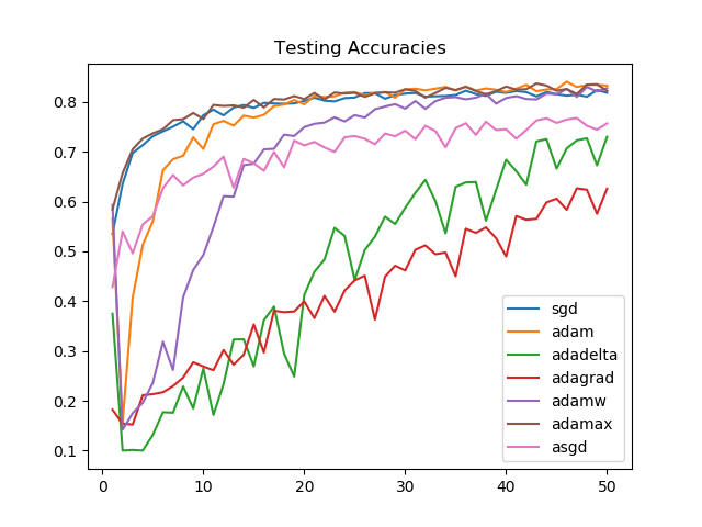
On unseen data, after 50 epochs, the model performance is similar for Adamax, SGD, Adam, and AdamW. The improvement in the first few epochs is the greatest for Adamax and SGD.

SGD and Adamax again see a consistently strong performance, as is reflected by the training accuracies as well.

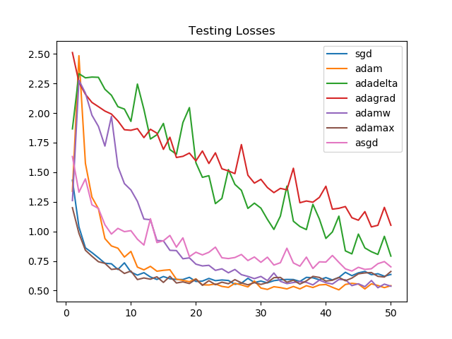
Losses on the validation set, though, see Adam and AdamW as victorious. For SGD and Adamax the losses increase towards the end, suggesting the need for an early stopping mechanism.

Looking at the graphs, it is clear that for the task we chose, Adagrad and Adadelta improve linearly and aren't able to perform as well as Adammax, SGD, Adam, or AdamW.

More Benchamrking of Optimizers

Other, lesser-known optimizers include:

1. QHAdam - Quasi-Hyperbolic Adam decouples the momentum update and the squared gradients update from the update mechanism, and instead uses a quasi-hyperbolic formulation. This uses a weighted average of current and previous gradients, discounted by a constant, and another weighted average of current and previous squared gradients, discounted by another constant, in the denominator.
2. YellowFin - In YellowFin, the learning rate and momentum values are tuned every iteration by minimizing a local quadratic function in a way that the tuned hyperparameters help maintain a constant convergence rate.  
3. Demon - Decaying Momentum is a momentum rule that can be applied to any gradient descent algorithm with momentum. The decaying momentum rule reduces the velocity value by decaying the "energy" that a gradient transfers to the future time step by weighting it with the ratio of current time step to the final time step. There is usually no hyperparameter tuning required because the momentum usually decays to 0 towards the final optimization iterations. The algorithm performs better when the decaying is delayed.

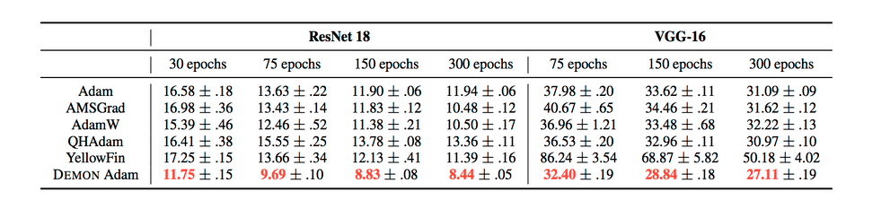
To dive more deeply into these slightly less popular gradient descent algorithms, check this article. To compare some of the above mentioned optimizers, they used 6 test problems:

1. CIFAR10 - ResNet18
2. CIFAR100 - VGG16
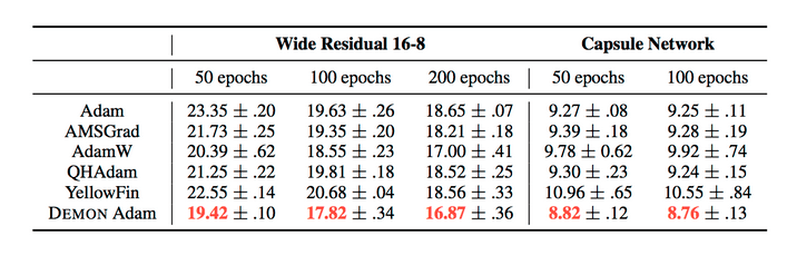
3. STL100 - Wide ResNet 16-8
4. FashionMNIST - CAPS
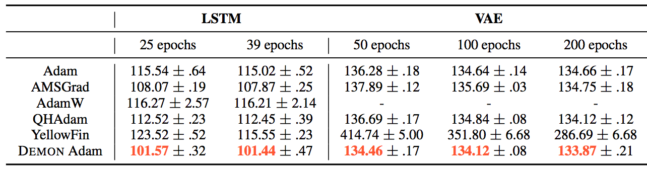
5. PTB - LSTM
6. MNIST - VAE

And tested the following Adaptive Learning Rate Optimizers:

1. Adam
2. AMSGrad
3. AdamW
4. QHAdam
5. YellowFin
6. Demon

The results can be summarized by the following tables:

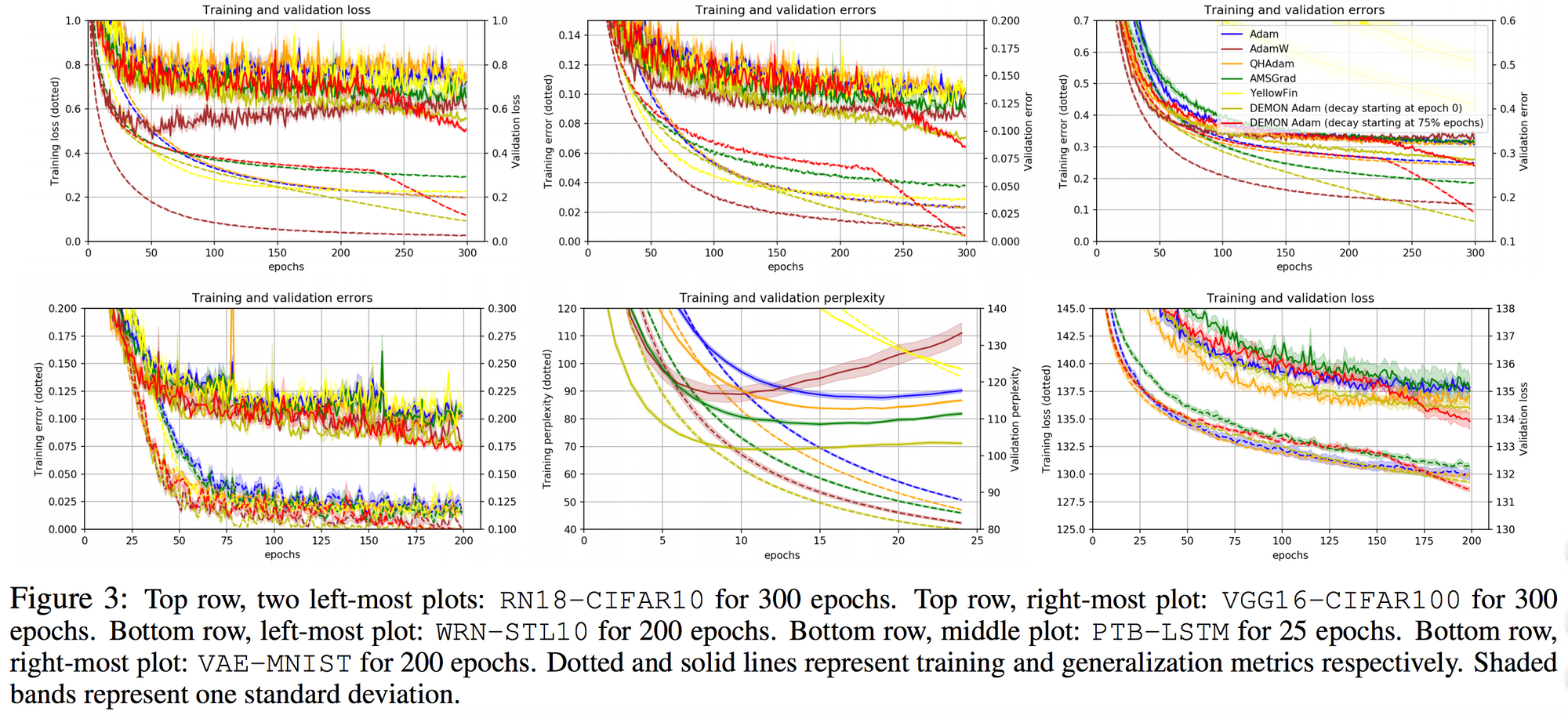
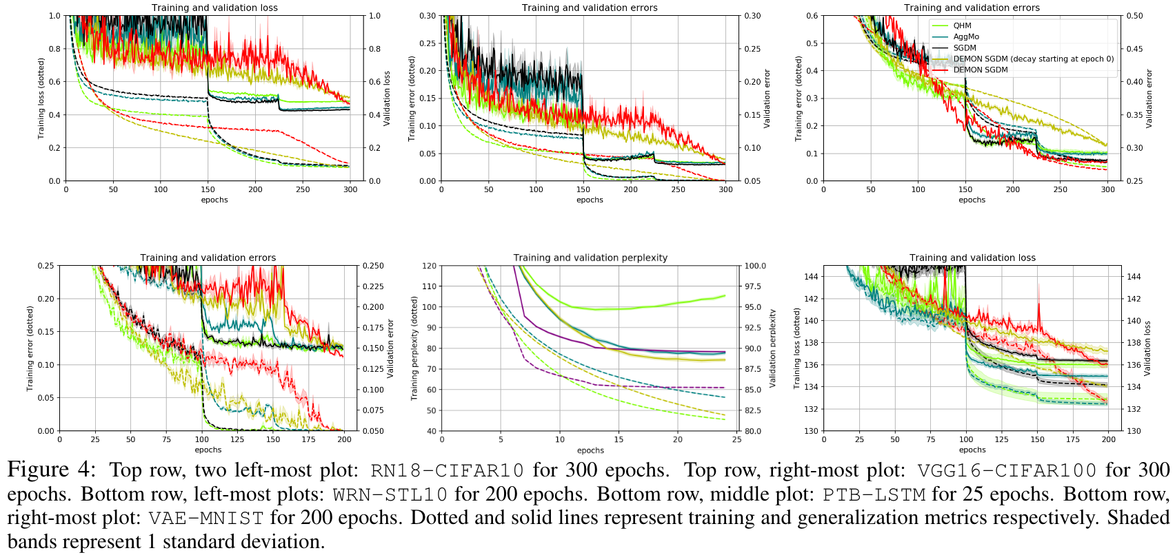
They also demonstrate the training and validation loss over several epochs in the following plots.

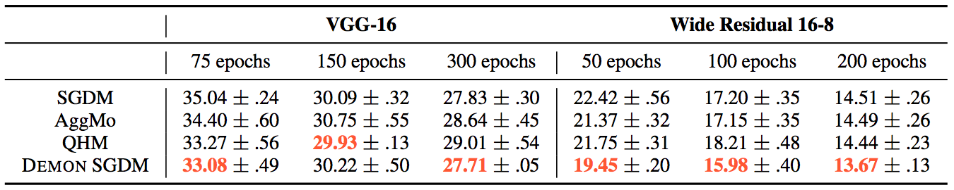
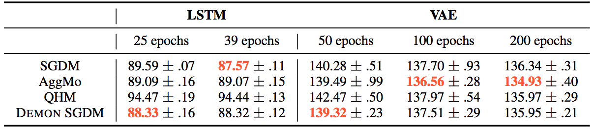
For the same tasks, they also tested non-adaptive learning rate optimizers, such as:

1. SGDM
2. AggMo
3. QHM
4. Demon SGDM

For the CIFAR10 - ResNet18 task, the results were:

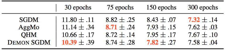
Whereas for the other tasks:

The loss plots looked like this:

There are also several other optimization methods, like methods based on genetic algorithms or probabilistic optimization methods like simulated annealing, that can serve as good replacements for gradient descent in certain contexts. In reinforcement learning, for example, there is a need for discrete optimization which can be done via several policy optimization algorithms. Some of the algorithms that build up on the classic REINFORCE algorithm can be found here.

Summary

We looked at gradient descent and implemented vanilla and momentum update mechanisms from scratch in Python. We also visualized our gradient updates on Ackley's function as movement along the contour plots. We benchmarked several optimizers for an image classification task using the CIFAR10 dataset, and trained a ResNet18 for this purpose. The results showed that Adamax, SGD, AdamW and Adam performed well, whereas Adagrad and Adadelta didn't. We then looked at several not-so-popular gradient descent-based optimizers which are currently being used in deep learning. In the end we looked at how several of the optimizers we discussed perform on different tasks, including tuning weights for convolutional architectures, LSTMs, and Variational Auto Encoders.