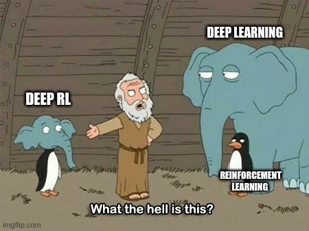
Deep Reinforcement Learning is one of the most quickly progressing sub-disciplines of Deep Learning right now. In less than a decade, researchers have used Deep RL to train agents that have outperformed professional human players in a wide variety of games, ranging from board games like Go to video games such as Atari Games and Dota. However, the learning barrier for Reinforcement Learning can be a bit daunting even for folks who have dabbled in other sub-disciplines of deep learning before (like computer vision and natural language processing).
In fact, that was exactly where I found myself when I started my current gig. I had the experience of working in computer vision for about 3 years, and suddenly I was thrown into Deep Reinforcement learning. It seemed like using neural networks to do stuff, but most of the recipes from standard deep learning did not work.
Almost a year down the line, I've finally come to appreciate the subtle nature of Reinforcement Learning (RL) , and thought it would be nice to write a post introducing the concepts of RL to people coming from a standard Machine Learning experience. I wanted to write this post in such a way that if someone making the switch (as I was, about a year ago) came across it, the article would serve as a good starting point and help shorten the time for the transition.
So let's get started.
In this post, we will cover:
- The Environment
- The State
- Markov Property
- Violations of the Markov Property in Real Life
- Partial Observability
- Markov Decision Processes
- The State
- Actions
- Transition Function
- Reward Function
- Partially Observable Markov Decision Processes
- Model-Based vs Model-Free Learning
- Model-Based Learning
- Model-Free Learning
Bring this project to life
The Environment
The first difference that one encounters upon switching to RL, and the most fundamental one, is that the neural network is trained through interactions with a dynamic environment instead of a static dataset. Normally you'd have a dataset that is made of up images/sentences/audio files and you would iterate over it, again and again, to get better at the task you are training for.
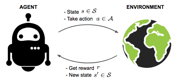
In RL, you have an environment in which you take actions. Each action fetches you a reward from the environment. The neural network (or any other function used to determine the actions) is called the agent. The lifespan of the agent may be finite (for example, games like Mario where the game terminates) or infinite (a perpetually continuing game). For now, we will only focus on RL tasks that terminate, and these are also called episodic tasks. RL tasks where the agent has an infinite lifespan will be tackled in the next part of this series.
The cumulative reward that the agent accumulates throughout the episode is called the return. The goal of reinforcement learning is to maximize this return. Solving this involves solving the credit assignment problem. It gets its name due to the fact that of all the possible actions we can take, we have to assign credit (return) to each action so that we can choose the one that yields the maximum return.
Technically, the goal of an RL agent is to maximize the expected return. But we will resist from dwelling much more on this aspect here. We will take it up in more detail in the next part where we will discuss RL algorithms in more detail. In this part, we restrict ourselves to a discussion of the central problems in RL.
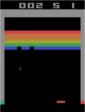
An example of an environment is the Atari game, Breakout.
In Breakout, the agent can move the slider left, right, or do nothing. These are the actions that the agent can execute. The environment rewards the agent when one of the bricks gets hit by the ball. The goal of doing RL is to train the agent so that all bricks are destroyed.
The State
The state of an environment basically gives us information about the environment. It can be a screenshot of the game, a series of screenshots, or a bunch of equations that govern how the environment works. In general, it is any information provided to the agent at each time step that helps it take an action.
Markov Property
If the information provided by the state is sufficient to determine the future states of the environment given any action, then the state is deemed to have the Markov property (or in some literature, the state is deemed as Markovian). This comes from the fact that the environments we deal with while doing Reinforcement Learning are modeled as Markov Decision Processes. We will cover these in detail in just a bit, but for now, understand that these are environments whose future states (for any actions) can be determined using the current state.
Consider the Atari game Breakout. If we consider a screenshot of the game at any point as the state, is it Markovian?
The answer is no, because just given the screenshot there is no way to ascertain which direction the ball is going in! Consider the following image.
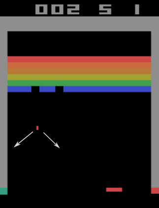
The ball could be going in either of the directions marked by the two white arrows, but we have no way to tell which. So maybe we need more information to make the state Markovian. How about we take the past 4 frames as our state, so that we have at least an idea of where the ball is heading?
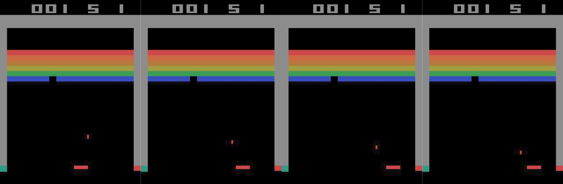
Given these 4 frames, we can compute the velocity as well as the direction of the ball to predict the future 4 frames (out of which the trailing 3 are the same as the leading 3 of the current state).
Environments can also be stochastic in nature. That is, given that the same action is applied to the same state, you could still end up in differing states as a result. If the probability distribution of the future states for all actions can be determined using the current state and current state alone, the state is termed as Markovian as well. This will become clearer when we go through the mathematical formulation of Markov Decision Processes in a bit.
Violations of the Markov Property in Real Life
Consider the case where we have to predict the future frame. Here, we have to predict at what angle the ball would bounce off.
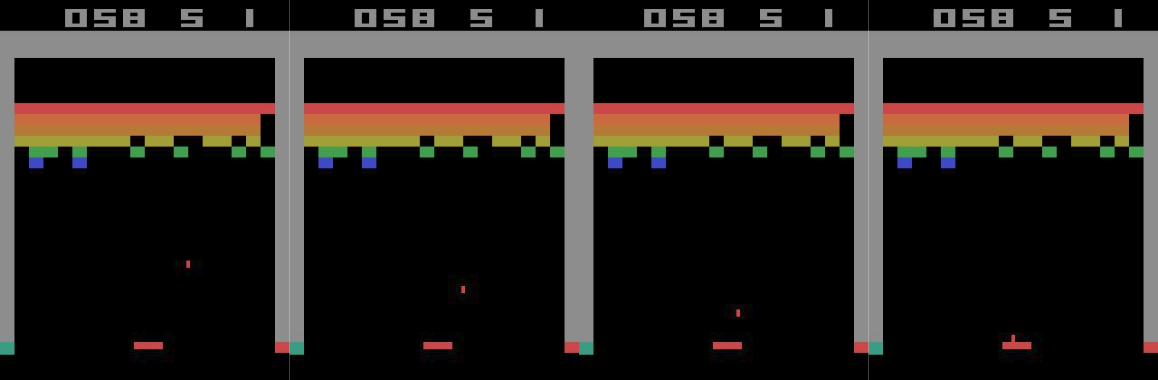
Of course, given the velocity and the angle of the ball, we could predict the angle and the velocity of the ball when it bounces off. However, that is only true when we assume that the system is ideal, and the collision between the ball and the disk is purely elastic.
If we were modeling such a scenario in real life, the non-elastic nature of the collision would violate the Markov property of the state. However, if we could add more details to the state such as the coefficient of restitution (something that will allow us to factor the non-elastic nature of the collision into our calculation), the state becomes Markovian again because we can precisely predict the future position of the ball. Thankfully, in Breakout, collisions are purely elastic.
It's very difficult to construct Markovian states for real-life environments. The first big hurdle is that sensors always add some noise to the readings, making it impossible to correctly predict (or even measure) the true state of the environment. Secondly, there are a lot of elements of the state which simply may not be known to us.
Consider a classic reinforcement learning task involving balancing a vertical pole. Here is a video of the real task.
The following excerpt is taken from a discussion of the Markov property in the famous book "Reinforcement Learning: An Introduction" by Barto and Sutton, which talks about the Markov property of the state in a pole-balancing experiment.
In the pole-balancing task introduced earlier, a state signal would be Markov if it specified exactly, or made it possible to reconstruct exactly, the position and velocity of the cart along the track, the angle between the cart and the pole, and the rate at which this angle is changing (the angular velocity). In an idealised cart–pole system, this information would be sufficient to exactly predict the future behaviour of the cart and pole, given the actions taken by the controller. In practice, however, it is never possible to know this information exactly because any real sensor would introduce some distortion and delay in its measurements. Furthermore, in any real cart–pole system there are always other effects, such as the bending of the pole, the temperatures of the wheel and pole bearings, and various forms of backlash, that slightly affect the behaviour of the system. These factors would cause violations of the Markov property if the state signal were only the positions and velocities of the cart and the pole.
Partial Observability
While it's hard to have states that have the Markov property, especially in real life, the good news is that approximations with near-Markov properties have worked well enough in practice for solving reinforcement learning tasks.
Consider the case of the pole-balancing experiment. A state that divided the position of the cart into three regions–right, left, and middle–and also used similarly rough-quantized values of intrinsic state variables (like the velocity of the cart, the angular velocity of the pole, etc.), worked well enough for the balancing problem to be solved through RL methods. Such a state is far from Markovian, but might have sped up learning by forcing the agent to ignore fine distinctions that would not have been useful in solving the task anyway.
While approaching the theoretical analysis of such environments, we assume that there indeed exists a state, often termed as merely "the state" or "the true state", with the Markov property that we cannot observe. What we can observe is only a part or a noisier version of the true state, which is called the observation. This is referred to as Partial Observability, and such environments are modeled as Partially Observable Markov Decision Processes (or simply POMDPs).
Note that there is some disparity in the literature in how states and observations are denoted. Some literature uses the word "state" for the true hidden state with the Markov property, whereas other literature would term the input to the neural network as the state, while referring to the hidden state with the Markov property as the "true state".
Now that we have established an understanding of the Markov property, let us define Markov Decision Processes formally.
Markov Decision Processes
Almost all problems in Reinforcement Learning are theoretically modelled as maximizing the return in a Markov Decision Process, or simply, an MDP. An MDP is characterized by 4 things:
- $ \mathcal{S} $ : The set of states that the agent experiences when interacting with the environment. The states are assumed to have the Markov property.
- $ \mathcal{A} $ : The set of legitimate actions that the agent can execute in the environment.
- $ \mathcal{P} $ : The transition function that governs which probability distribution of the states the environment will transition into, given the initial state and the action applied to it.
- $ \mathcal{R} $ : The reward function that determines what reward the agent will get when it transitions from one state to another using a particular action.
A Markov decision process is often denoted as $ \mathcal{M} = \langle \mathcal{S}, \mathcal{A}, \mathcal{P}, \mathcal{R} \rangle $. Let us now look into them in a bit more detail.
The State
The set of states, $ \mathcal{S} $, corresponds to the states that we discussed in the section above. States can be either a finite or an infinite set. They can be either discrete or continuous in measurement. $ \mathcal{S} $ describes the legitimate values the state of an MDP can take, and thus, is also referred as the state space.
An example of a finite discrete state space is the state we used for the Breakout game, i.e. the past 4 frames. The state consists of 4 210 x 160 images concatenated channel-wise, thus making the state an array of 4 x 210 x 160 integers. Each pixel can take values from 0 to 255. Therefore, the number of possible states in the state space is $ 255^{4 * 210 * 160} $. It's a huge but finite state space.
An example of a continuous state space is that of the CartPole-v0 environment in OpenAI Gym, which is based on solving the inverted pendulum task.
The state is made up of 4 intrinsic state variables: cart position, velocity, pole angle, and pole velocity at the tip. The following are legitimate values for the state variables.
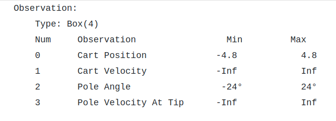
The state space is infinite since the continuous variables can take arbitrary values between the bounds.
Actions
The action space $ \mathcal{A} $ describes the legitimate actions that the agent can execute in the MDP. The actions transition the environment to a different state and the agent gets a reward after this transition.
Just like state spaces, action spaces are the basically the the range of legitimate actions. They can be either discrete like the action space of the Breakout game, which is [NO-OP, FIRE, RIGHT, LEFT], which makes the slider do nothing, fire the ball, move right or left respectively. A continuous action space can be that of a car racing game where the acceleration is the action that the agent can execute. This acceleration can be a continuous variable ranging from say, $ -3 m/s^2 $ to $ 3 m/s^2 $.
Transition Function
Transition function gives us the probability over the state space which describes the likelihood of the environment transitioning into various states given an action $ a $ is applied to the environment when it is in state $ s $. The function $ \mathcal{P}: \mathcal{S} \times \mathcal{A} \rightarrow \mathcal{S} $ gives us the probability distribution over future states.
$$ P_{ss'}^a = P(s' \vert s, a) = \mathbb{P} [S_{t+1} = s' \vert S_t = s, A_t = a] $$
The probability distribution of the future states of the Atari game Breakout, will be defined over $ 255^{4 * 210 * 160} $ states. In practice, computing such a distribution is often intractable, and we will see how such situations are tackled later in this post.
The form of the transition function is what endows the Markov property on the states of the MDP. The function is defined to produce a distribution over the future states $ s' $, given the current states $ s $ and the action applied $ a $ only. If the transition function were to require a history of states and actions, then the states would cease to have the Markov property.
Therefore, the Markov property is also expressed in mathematical terms as follows:
$$ \mathbb{P} [S_{t+1} = s' \vert S_t = s, A_t = a] = \mathbb{P} [S_{t+1} = s' \vert S_t , a_t, S_{t-1}, a_{t-1} .... S_0, a_0] $$
That is, all you need is the current state and action to define a distribution over future states regardless of the history of that states visited and actions taken by the agent.
Reward Function
Reward function tells us what reward will the agent get if it takes action $a$ in the state $ s_t $. The function $ \mathcal {R} : \mathcal {S} \times \mathcal {A}\rightarrow \mathbb{R} $ that provides us with the reward agent gets on taking a particular action in a particular state.
$$ R(s, a) = \mathbb{E} [R_{t+1} \vert S_t = s, A_t = a] $$
Partially Observable Markov Decision Processes
It is not hard to extend theoretical framework of MDPs to define a Partially Observable MDP, or POMDP. A POMDP is defined as $ \mathcal{M} = \langle \mathcal{S}, \mathcal{A}, \mathcal{P}, \mathcal{R}, \Omega, \mathcal{O} \rangle $
In addition to $\mathcal{S}, \mathcal{A}, \mathcal{P}, \mathcal{R}, $we define:
- $ \Omega $, a set which describes the legitimate values for the observations.
- Conditional observation function $ O (s', a) $ which tells us the distribution over the observations the agent will receive if the agent has taken the action $ a $ to transition into the new state $ s' $.
Model v/s Model Free Learning
As we discussed, for the game Breakout, our state is an extremely high dimensional one, having dimensions of $ 255 ^ {4 * 210 * 160} $. With such a high state, the transition function needs to output a distribution over these many states. As you may have figured out, doing that is intractable with the current hardware capabilities, and remember, the transition probabilities needs to be computed at every step.
There are a couple of ways to circumvent this issue.
Model Based Learning
We could either spend our efforts in trying to learn a model of the the breakout game itself. This would involve using deep learning to learn the transition function $ /mathcal{P} $ and reward function $ \mathcal{R} $. We could model the state as a 4 x 210 x 160-dimensional continuous space where each dimension ranges from 0 to 255 and come up with a generative model.
When we learn these things, it is said we are learning the model of the environment. We use this model to learn a function called the policy, $ \pi: \mathcal{S} \times \mathcal{A} \rightarrow [0,1] $, which basically gives us the agent the probability distribution $ \pi(s,a) $ over actions $ a$ to take when it experiences a state $ s $.
Generally, learning an optimal policy (one that maximizes the return) when you have a model of the environment is termed as planning. RL methods that learn the model of the environment in order to arrive at the optimal policy are categorised under Model-based Reinforcement Learning.
Model Free Learning
Alternatively, we could find that the underlying environment is too hard to model, and maybe it is better to learn directly from experiences rather than trying to learn the model of the environment before.
This is similar to how humans learn most of their tasks too. The driver of the car doesn't actually learn the laws of physics that govern the car, but learns to make decisions on basis of his experience of how the car reacts to different actions ( The car skids if you try to accelerate is too quickly etc).
We can also train our policy $ \pi $ this way. Such a task is termed as a Control task. RL methods which try to learn optimal policies for control tasks directly from experience are categorised as Model-free Reinforcement Learning.
Wrapping up
That is it for this part. This part was about setting up the problem, trying to give you a feel about the framework of problems we deal with in reinforcement learning, first through intuition and then through maths.
In the next part, we will tackle on how these tasks are solved and the challenges we face while applying techniques borrowed from standard deep learning. Till then, here are a few resource to further dwelve in the material covered in this post!
- Chapter 3, Reinforcement Learning: An Introduction by Barto & Sutton.
- RL Course by David Silver - Lecture 2: Markov Decision Process