This article is about one of the revolutionary GANs, ProGAN from the paper Progressive Growing of GANs for Improved Quality, Stability, and Variation. We will go over it, see its goals, the loss function, results, implementation details, and break down its components to understand each of these. If we want to see the implementation of it from scratch, check out this blog, where we replicate the original paper as close as possible, and make an implementation clean, simple, and readable using PyTorch.
If we are already familiar with GANs and know how they work, continue through this article, but if not, it's recommended to check out this blog post first.
Gan Improvements
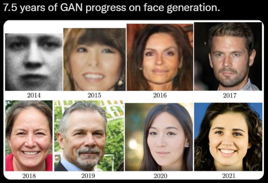
In this section, We will learn about GAN improvements. We will see how GANs have advanced over time. In the figure above we can see a visualization of the rate at which GANs have improved over the years.
- In 2014 Ian Goodfellow gave machines the gift of imagination by creating the powerful AI concept of GANs from the paper Generative Adversarial Networks, but they were incredibly sensitive to hyperparameters, and the generated images looked low-quality. We can see the first face which is black and white and looks barely like a face. We can read about the original GANs in these blogs: Discover why GANs are awesome!, Complete Guide to Generative Adversarial Networks (GANs), and Building a simple Generative Adversarial Network (GAN) using TensorFlow.
- Since then researchers start to improve GANs, and in 2015 a new method was introduced, DCGANs from the paper Unsupervised Representation Learning with Deep Convolutional Generative Adversarial Networks. We can see in the second image, that the face looks better but it's still far from perfection. We can read about it in this blog: Getting Started With DCGANs.
- Next in 2016, CoGAN, from the paper Coupled Generative Adversarial Networks was introduced, which improved face generation even further.
- At the end of 2017, researchers from NVIDIA AI released ProGAN along with the paper Progressive Growing of GANs for Improved Quality, Stability, and Variation, which is the main subject of this article. We can see that the fourth picture looks more realistic than the previous ones.
- In 2018 the same researchers come up with StyleGAN from the paper A Style-Based Generator Architecture for Generative Adversarial Networks, which is based on ProGAN. We will cover it in an upcoming article. We can see the high-quality faces that StyleGAN can generate and how realistic they look.
- In 2019 the same researchers again come up with StyleGAN2 from the paper Analyzing and Improving the Image Quality of StyleGAN which is an improvement over StyleGAN. In 2021, again they come up with StyleGAN3 from the paper Alias-Free Generative Adversarial Networks, which is an improvement over StyleGAN2. We will cover both of them in upcoming articles separately, break down their components and understand them, then implement them from scratch using PyTorch.
StyleGan3 is the king in image generation, it beat other GANs out of the water on quantitative and qualitative evaluation metrics, both when it comes to fidelity and diversity.
Because of these papers and others, GANs have advanced largely from improved training, stability, capacity, and diversity.
ProGAN Overview
In this section, we will learn about ProGAN's relatively new architecture that's considered an inflection point improvement in GAN. We will go over ProGAN's primary goals and get an introduction to its architecture in individual components.
ProGAN goals
- Produce high-quality, high-resolution images.
- Greater diversity of images in the output.
- Improve stability in GANs.
- Increase variation in the generated images.
Main components of ProGAN
Traditional Generative adversarial networks have two components; the generator and the discriminator. The generator network takes a random latent vector (z∈Z) and tries to generate a realistic image. The discriminator network tries to differentiate real images from generated ones. When we train the two networks together the generator starts generating images indistinguishable from real ones.
In ProGAN the key idea is to grow both the generator and discrimination progressively, The generator starts with learning to generate a very small input image of 4x4, and then when it has achieved that task, where the target images look very close to the generated images so the discriminator can't distinguish between them at this specific resolution, then we update it, and the generator generates 8x8 images. When it's finished with that challenge, we upgrade it again to 16x16, and we can imagine this continuing until eventually reach 1024 x 1024 pixel images.
This idea just makes sense because it's similar to the way that we learn. If we take mathematics, for example, we don't ask on day 1 to calculate gradients; we start from the foundation doing simple addition, and then we are progressively grown to do more challenging tasks. This is the key idea in ProGAN, but additionally, the authors also describe several implementation details that are important and they are Minibatch Standard Deviation, Fading in new layers, and Normalization (PixelNorm & Eq. LR). Now let's get a deeper dive into each of these components and how they work.
Progressive Growing
In this section, we will learn about progressive growing, which is the key idea of ProGAN. We will go over both the intuition behind it as well as the motivation and then we will dive a little bit deeper into how to implement it.
First off, progressive growing is trying to make it easier for the generator to generate higher resolution images by gradually training it from lower resolution images to higher resolution images. Starting with an easier task, a very blurry image for it to generate a 4x4 image with only 16 pixels to then a much higher resolution image over time.
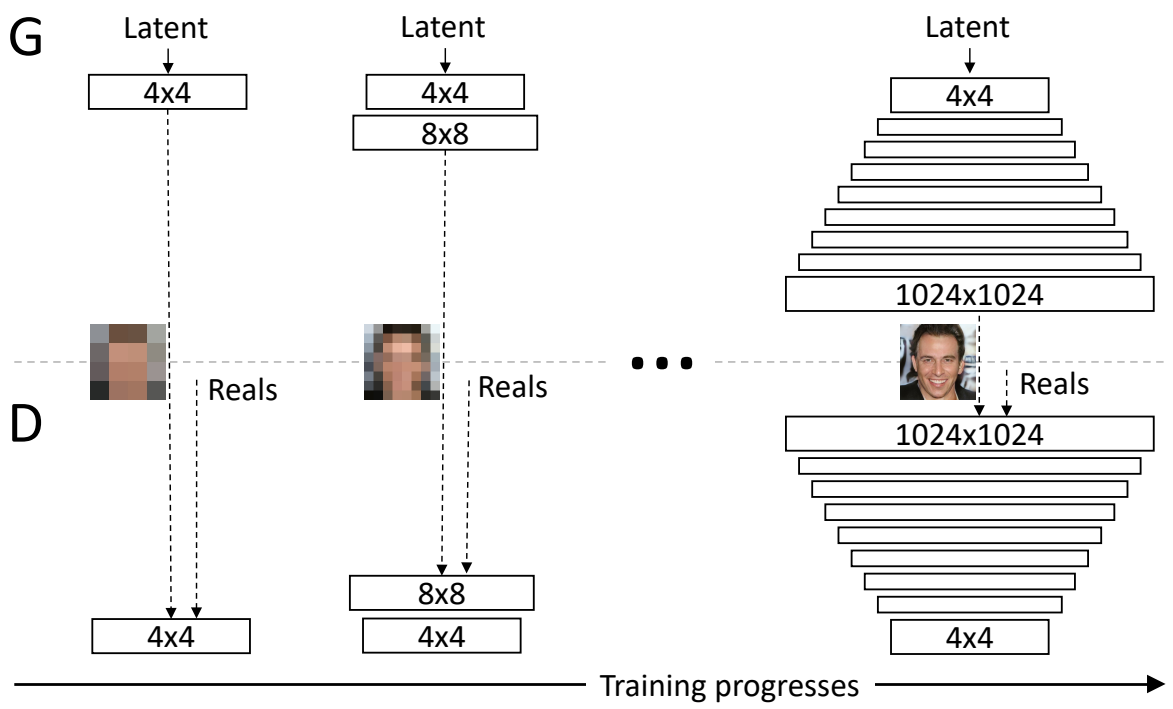
First, the generator just needs to generate a four-by-four image and the discriminator needs to evaluate whether it's real or fake. Of course, to make it not so obvious what's real or fake, the real images will also be downsampled to a four-by-four image. In the next step of progressive growing, everything is doubled, so the image now generated is an eight-by-eight image. It's of a much higher resolution image than before, but still an easier task than a super high-resolution image, and of course, the reals are also down-sampled to an eight-by-eight image to make it not so obvious which ones are real and which ones are fake. Following this chain, the generator is eventually able to generate super high-resolution images, and the discriminator will look at that higher resolution image against real images that will also be at this high resolution, so no longer downsampled and be able to detect whether it's real or fake.
In the image below, we can see progressive growing in action from really pixelated four-by-four pixels to super-high-resolution images.
Minibatch Standard Deviation
GANs have a tendency to not show as varied images as in training data, so the authors of ProGAN solve this issue with a simple approach. They first compute the standard deviation for every example across all of the channels and all of the pixel values, and then they take a mean across all of over the batch. Then they replicate that value (which is just a single scalar value) across all of the examples and then all of the pixel values to get a single channel, and concatenate it to the input.
Fading in new layers
By now, we should understand how, in ProGANs, we do progressive growing where we start by 4x4, then 8x8, etc. But this progressive growing isn't as straightforward as just doubling in size immediately at these scheduled intervals, it's actually a little bit more gradual than that.
For the generator
When we want to generate a double-size image, first we upsample the image (upsampling could use techniques like nearest neighbors filtering). Without using any learned parameters it's just very basic upsampling, and then in the next step we could do 99% upsampling and 1% of taking the upsampled image into a convolutional layer that produces a double size resolution image, so we have some learned parameters.
Over time we start to decrease the percentage of upsampling, and increase the percentage of learned parameters, so the image starts to look perhaps more like the target (I.e face, if we want to generate faces), and less like just upsampling from nearest neighbors upsampling. Over time, the model will begin to rely not on the upsampling, but instead just rely on learned parameters for inference.
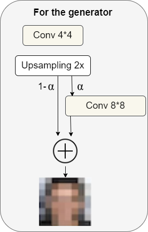
More generally, we can think of this as an α parameter that grows over time, where α starts out as 0 and then grows all the way up to 1. We can write the final formulation as follows: $[(1−α)×UpsampledLayer+(α)×ConvLayer]$
For the discriminator
For the discriminator, there's something fairly similar, but in the opposite direction.
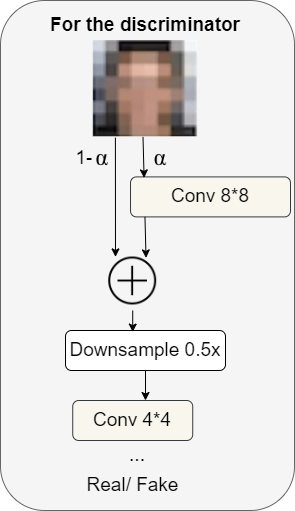
We have a high-resolution image (example: 8x8 in the figure above), and slowly over time, we go through the downsampling layer to then handle the low-resolution image (exp: 4x4 in the figure above). At the very end, we output a probability between zero and one (real or fake) corresponding to the prediction.
The α that we use in the discriminator is the same that we saw in the generator.
Normalization
Most if not all earlier advanced GANs use batch normalization in the generator and in the discriminator to eliminate covariate shift. But the authors of ProGAN observed that this is not an issue in GANs and they use a different approach that consists of a two-step process.
Equalized Learning Rate
Because of the problem with optimizers which is the gradient update steps in Adam and RMSProp depending upon the dynamic range of the parameters, the authors of ProGAN introduced their solution, the Equalized learning rate, to better solve for their specific problem.
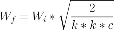
Before every forward pass, learning rates can be equalized across layers by scaling the weights. For example, before performing a convolution with f filters of size (k, k, c), they scale the weights of those filters as shown below. In that way, they ensure that every weight is in the same dynamic range, and then the learning speed is the same for all weights.
Pixel Normalization
To get rid of batch normalization, the authors applied pixel normalization after the convolutional layers in the generator to prevent signal magnitudes from spiraling out of control during training.
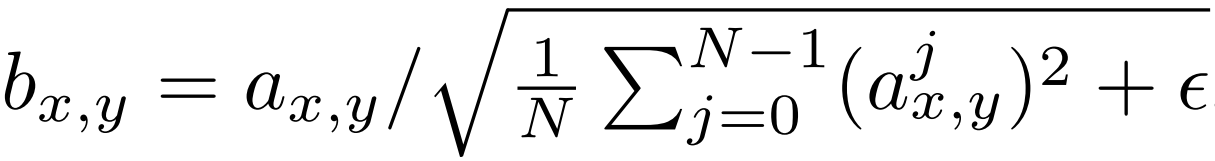
Mathematically the new feature vector in pixel (x,y) will be the old one divided by the square root of the mean of all pixel values squared for that particular location plus epsilon that equals 10^-8. The implementation of this is going to be pretty clear (You can see the whole implementation of ProGAN from scratch in this blog).
The Loss Function
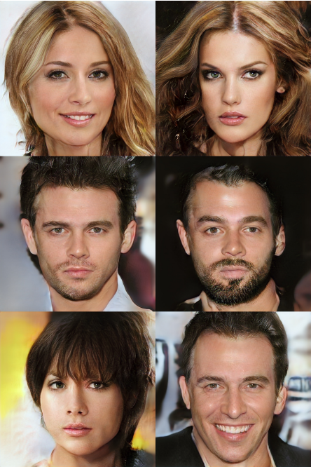
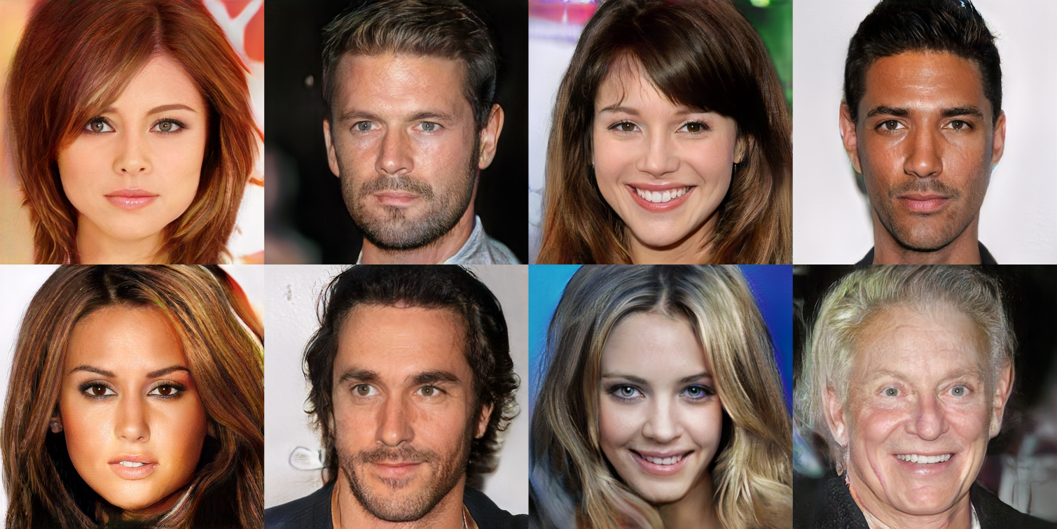
For the loss function, the authors use one of the common loss functions in GANs, the Wasserstein loss function, also known as WGAN-GP from the paper Improved Training of Wasserstein GANs. But, they also say that the choice of the loss function is orthogonal to their contribution, which means that none of the components of ProGAN (Minibatch Standard Deviation, Fading in new layers, and Normalization (PixelNorm & Eq. LR)) rely on a specific loss function. It would therefore be reasonable to use any of the GAN loss functions we want, and they demonstrate so by training the same network using LSGAN loss instead of WGAN-GP loss. The figure below shows six examples of 10242 images produced using their method using LSGAN.
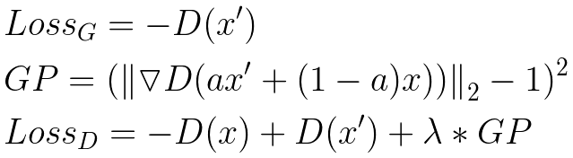
However, we are trying to follow the paper exactly so let's explain WGAN-GP a little bit. In the figure below, we can see the loss equations where:
- x’ is the generated image.
- x is an image from the training set.
- D is the discriminator.
- GP is a gradient penalty that helps stabilize training.
- The a term in the gradient penalty refers to a tensor of random numbers between 0 and 1, chosen uniformly at random.
- The parameter λ is common to set to 10.
Results
I think the results are surprising for most people, they look very good, they are 1024 by 1024 images and they are a lot better than the previous ones. So this is one of those revolutionary papers that was the first to generate really high-quality images in GANs.
Implementation details
The authors train the network on eight tesla v100 GPUs until they didn't observe any sort of improvements. This took about four days. In their implementation, they used an adaptive minibatch size depending on the output resolution, so that the available memory budget was optimally utilized (they decreased the batch size when they couldn't hold that into the memory).
Generator
In traditional GANs we ask the generator to generate immediately a fixed resolution, like 128 by 128. Generally speaking, higher resolution images are much more difficult to generate, and it's a kind of a challenging task to directly output high-quality images. In ProGAN we ask the generator to:
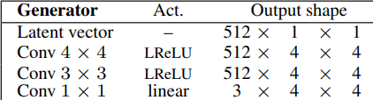
- First, generate four by four images by taking as input a latent vector equal to 512. They can also name it noise vector or z-dim, then map it to 512 (in 1 channels). Then, they follow a nice trend, where they use a transposed convolution that maps one by one to four by four in the beginning, followed by the same convolution with three by three filter, using leaky ReLU as activation function in both convolutions. Finally,, they add a one by one convolution that maps the number of channels which is 512 to RGB (3 channels).
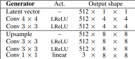
- Next, they Generate eight by eight images by using the same architecture without the final convolution layer that maps the number of channels to RGB. Then, they add the following layers: upsampling to double the previous resolution, two Conv layers with three by three filter using leaky ReLU as activation function, and another Conv layer with one by one filter to output an RGB image.
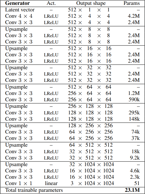
- Then, they again generate double the size of the previous one by using the same architecture without the last convolution layer and adding the same layers (upsampling to double the previous resolution, two Conv layers with three by three filter using leaky ReLU as activation function, and another Conv layer with one by one filter to output an RGB image.) until reaching the resolution desired: 1024 x 1024. In the image below, we can see the final architecture of the generator.
Discriminator
For the discriminator, they do an opposite approach. It's sort of a mirror image of the generator. When we try to generate a current resolution, we downsample the real images to the same resolution to not make it so obvious what's real or fake.
- They start by generating four-by-four images, which means downsampling the real images until reaching the same resolution. The input of the discriminator is the RGB images we do three Conv layers the first with one-by-one filter, and the others with three-by-three filters, using leaky ReLU as an activation function. We then downsample the image to half the previous current resolution, and add two Conv layers with three-by-three filter and Leaky Relu. Then we downsample again, and so on until we reach the resolution that we want. Then, we inject Minibatch Standard Deviation as a feature map, so it goes from the number of channels to the number of channels + 1 (In this case 512 to 513). They can then run it through the last two Conv layers with 3x3 and 4x4 filters respectively. And in the end, they have a full connected layer to map the number of channels (512) to one channel. In the figure below, we can see the discriminator architecture for four-by-four images.
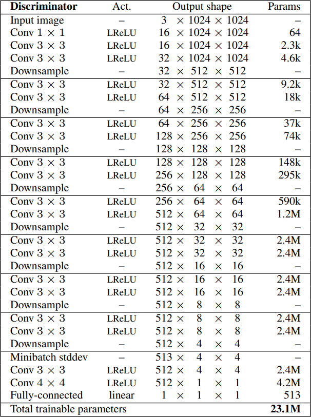
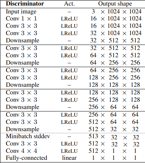
- If we want to generate X-by-X images (in which X is the resolution of the images) we just use the same steps as previous until we reach the resolution that we want, then we add the final four layers(Minibatch STddev, Conv 3x3x, Conv 4x4, and Fully connected). In the figure below, we can see the discriminator architecture for 32x32 images.
Conclusion
In this article, we looked at some of the major milestones in the developmental history of GANs, and went through the revolutionary ProGAN paper that was the first to generate really high-quality images. We then explored the original model's goals, the loss function, results, implementation details, and its components to help understand these networks in depth.
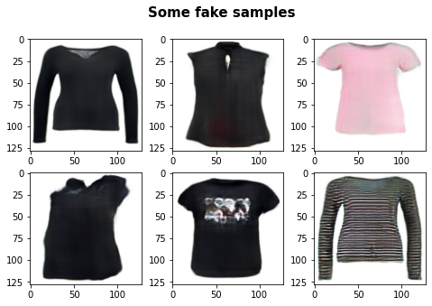
Hopefully, readers are able to follow all of the steps and get a good understanding of it, and get ready to tackle the implementation. We can find it in this article where we made a clean, simple, and readable implementation of the model to generate some fashion instead of faces, using this dataset from Kaggle for training. In the figure below you can see the results that we gain for resolution 128x128.
In upcoming articles, we will explain and implement from scratch StyleGANs using PyTorch (StyleGAN1 which is based on ProGAN, StyleGAN2 which is an improvement over SyleGAN1, and StyleGAN3 which is an improvement over SyleGAN2) to generate also some cool fashion.