Implementation of ProGAN from scratch

ProGAN from the paper Progressive Growing of GANs for Improved Quality, Stability, and Variation is one of the revolutionary papers that was the first to generate really high-quality images. In this article, we will make a clean, simple, and readable implementation of it using PyTorch. (If you prefer TensorFlow/Keras you can see this amazing article written by Bharath K.)  We will try to replicate the original paper as closely as possible, so if you read the paper the implementation should be pretty much identical.

If you don't read the ProGan paper or don't know how it works and you want to understand it I highly recommend you to check out this post blog where I go throw the details of it. And if you are new to GANs you can start with this article where I explain why GANs are awesome, understand what GANs really are, how they work, dive deep into the loss function that they use, and then build a simple GAN from scratch to generate MNIST.

The dataset that we will use in this blog is this dataset from Kaggle which contains 16240 upper clothes for women with 256*192 resolution. It's really a small dataset with low resolution compared to the one that the authors of ProGAN use which contains 800k images with high resolution 1024*1024 but it still gives us good results. You can try to use a better dataset to get better-generated images of any kind you want (faces, cars, houses,...).

Now let's start by loading the necessary libraries.

Load all dependencies we need

We first will import torch since we will use PyTorch, and from there we import nn. That will help us create and train the networks, and also let us import optim, a package that implements various optimization algorithms (e.g. sgd, adam,..). From torchvision we import datasets and transforms to prepare the data and apply some transforms.

We will import functional as F from torch.nn to upsample the images using interpolate, DataLoader from torch.utils.data to create mini-batch sizes, save_image from torchvision.utils to save some fake samples, and log2 form math because we need the inverse representation of the power of 2 to implement the adaptive minibatch size depending on the output resolution, Numpy for linear algebra, os for interaction with the operating system, tqdm to show progress bars, and finally matplotlib.pyplot to show the results and compare them with the real ones.

import torch
from torch import nn, optim
from torchvision import datasets, transforms
import torch.nn.functional as F
from torch.utils.data import DataLoader
from torchvision.utils import save_image
from math import log2
import numpy as np
import os
from tqdm import tqdm
import matplotlib.pyplot as plt

Seed everything

Let's seed everything to make results somewhat reproducible

def seed_everything(seed=42):
    os.environ['PYTHONHASHSEED'] = str(seed)
    np.random.seed(seed)
    torch.manual_seed(seed)
    torch.cuda.manual_seed(seed)
    torch.cuda.manual_seed_all(seed)
    torch.backends.cudnn.deterministic = True
    torch.backends.cudnn.benchmark = False
seed_everything()

Hyperparameters

• Initialize the DATASET by the path of the real images.
• Specify the start train at image size four by four as the paper.
• Initialize the device by Cuda if it is available and CPU otherwise, and learning rate by 0.001.
• The batch size will be different depending on the resolution of the images that we want to generate, so we initialize BATCH_SIZES by a list of numbers, you can change them depending on your VRAM.
• Initialize image_size by 128 and CHANNELS_IMG by 3 because we will generate 128  by 128 RGB images.
• In the original paper, they initialize Z_DIM and IN_CHANNELS by 512, but I initialize them by 256 instead for less VRAM usage and speed-up training. We could perhaps even get better results if we doubled them.
• For ProGAN we can use any of the GANs loss functions we want but we are looking to follow the paper exactly, so we will use the same loss function as they used the Wasserstein loss function, also known as WGAN-GP from the paper Improved Training of Wasserstein GANs. This loss contains a parameter name λ and it's common to set λ = 10.
• Initialize PROGRESSIVE_EPOCHS by 30 for each image size.

DATASET                 = "Women clothes"
START_TRAIN_AT_IMG_SIZE = 4
DEVICE                  = "cuda" if torch.cuda.is_available() else "cpu"
LEARNING_RATE           = 1e-3
BATCH_SIZES             = [32, 32, 32, 16, 16, 16] #you can use [32, 32, 32, 16, 16, 16, 16, 8, 4] for example if you want to train until 1024x1024, but again this numbers depend on your vram
image_size              = 128
CHANNELS_IMG            = 3
Z_DIM                   = 256  # should be 512 in original paper
IN_CHANNELS             = 256  # should be 512 in original paper
LAMBDA_GP               = 10
PROGRESSIVE_EPOCHS      = [30] * len(BATCH_SIZES)

Get and check the Data loader

Now let's create a function get_loader to:

• Apply some transformation to the images (resize the images to the resolution that we want, convert them to tensors, then apply some augmentation, and finally normalize them to be all the pixels ranging from -1 to 1).
• Identify the current batch size using the list BATCH_SIZES, and take as an index the integer number of the inverse representation of the power of 2 of image_size/4. And this is actually how we implement the adaptive minibatch size depending on the output resolution.
• Prepare the dataset we use ImageFolder because it's already structured in a nice way.
• Create mini-batch sizes using DataLoader that take the dataset and batch size with shuffling the data.
• Finally, return the loader and dataset.

def get_loader(image_size):
    transform = transforms.Compose(
        [
            transforms.Resize((image_size, image_size)),
            transforms.ToTensor(),
            transforms.RandomHorizontalFlip(p=0.5),
            transforms.Normalize(
                [0.5 for _ in range(CHANNELS_IMG)],
                [0.5 for _ in range(CHANNELS_IMG)],
            ),a
        ]
    )
    batch_size = BATCH_SIZES[int(log2(image_size / 4))]
    dataset = datasets.ImageFolder(root=DATASET, transform=transform)
    loader = DataLoader(
        dataset,
        batch_size=batch_size,
        shuffle=True,
    )
    return loader, dataset

Now let's check if everything works fine and see what the real images look like.

def check_loader():
    loader,_ = get_loader(128)
    cloth ,_ = next(iter(loader))
    _, ax    = plt.subplots(3,3, figsize=(8,8))
    plt.suptitle('Some real samples', fontsize=15, fontweight='bold')
    ind = 0 
    for k in range(3):
        for kk in range(3):
            ind += 1
            ax[k][kk].imshow((cloth[ind].permute(1,2,0)+1)/2) 
check_loader()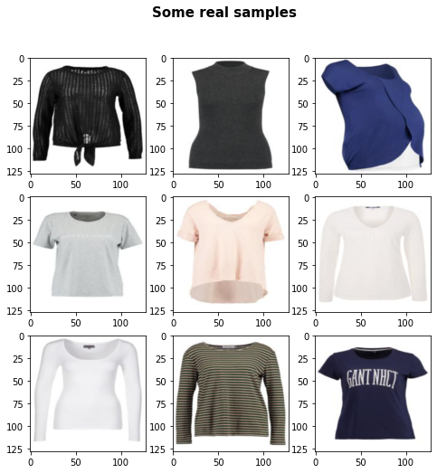

Models implementation

Now let's Implement the ProGAN generator and discriminator with the key attributions from the paper. We will try to make the implementation compact but also keep it readable and understandable. Specifically, the key points:

• Progressive growing (of model and layers)
• Minibatch std on Discriminator
• Normalization with PixelNorm
• Equalized Learning Rate

We explain all these key points in detail in this article.

Most of the tricky parts are in the implementation of the models. So this is definitely going to be the hardest part of this tutorial, this is why I am asking you to be a little bit more focused and patient.

Let's begin by building the generator.

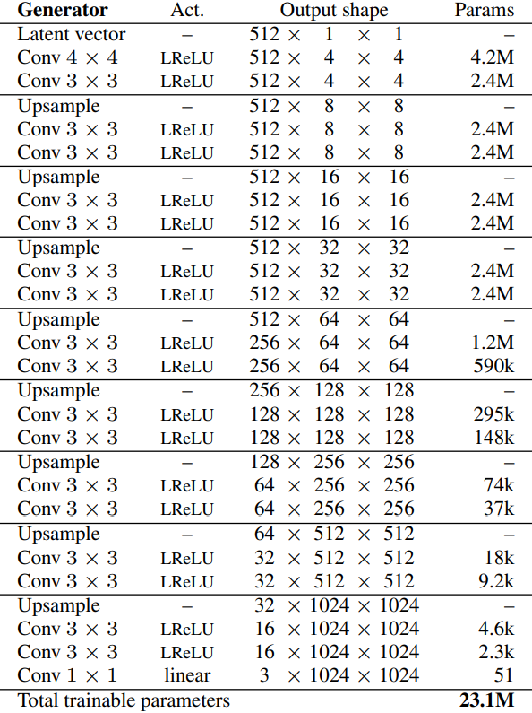
In the figure above, we can see the architecture of the generator. For the number of channels, we have 512 (256 in our case) four-time, then we decrease it by 1/2, 1/4, etc. Let's define a variable with the name factors which will be used in Discrmininator and Generator for how much the channels should be multiplied and expanded for each layer.

factors = [1, 1, 1, 1, 1 / 2, 1 / 4, 1 / 8, 1 / 16, 1 / 32]

Equalized Learning Rate

Now let's implement Equalized Learning Rate for the generator, let's name the class WSConv2d (weighted scaled convolutional layer) which will be inherited from nn.Module.

• In the init part we send in_channels, out_channels, kernel_size, stride, and padding. We use all of that to do a normal Conv layer, then we define a scale that will be the same as the function part2 in the figure below, we copy the bias of the current column layer into a variable because we don't want the bias of the convolution layer to be scaled, then we remove it, Finally, we initialize conv layer.  

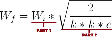
• In the forward part, we send x and all that we are going to do is multiplicate x with scale and add the bias after reshaping it.

class WSConv2d(nn.Module):

    def __init__(
        self, in_channels, out_channels, kernel_size=3, stride=1, padding=1,
    ):
        super(WSConv2d, self).__init__()
        self.conv      = nn.Conv2d(in_channels, out_channels, kernel_size, stride, padding)
        self.scale     = (2 / (in_channels * (kernel_size ** 2))) ** 0.5
        self.bias      = self.conv.bias #Copy the bias of the current column layer
        self.conv.bias = None      #Remove the bias

        # initialize conv layer
        nn.init.normal_(self.conv.weight)
        nn.init.zeros_(self.bias)

    def forward(self, x):
        return self.conv(x * self.scale) + self.bias.view(1, self.bias.shape[0], 1, 1)

Normalization with PixelNorm

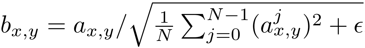
Now let's create a class for PixelNorm, for normalization.

• In the init part we define epsilon by 10^-8.
• In the forward part, we send x, and we return the same as the function in the figure below.

class PixelNorm(nn.Module):
    def __init__(self):
        super(PixelNorm, self).__init__()
        self.epsilon = 1e-8

    def forward(self, x):
        return x / torch.sqrt(torch.mean(x ** 2, dim=1, keepdim=True) + self.epsilon)

ConvBlock

If you noticed in the Generator architecture they repeat two convolution layers with three by three filters a bunch of times, so let's make them in a separate class to make the code cleaner, and actually, we are going to use it in the discriminator as well, the only difference between the two is that the discriminator we will not use pixel norm.

• In the init part we send in_channels, out_channels, and use_pixelnorm, then we initialize conv1 by WSConv2d which maps in_channels to out_channels, conv2 by WSConv2d which maps out_channels to out_channels, leaky by Leaky ReLU with a slope of 0.2 as they use in the paper, pn by PixelNorm(The last block that we create), and  use_pn by use_pixelnorm to specify if we are using PixelNorm or not.
• In the forward part, we send x, and we pass it to conv1 with leaky, then we normalize it with pn (PixelNorm) if use_pixelnorm is True, otherwise, we don't, and again we pass that into conv2 with leaky and we normalize it if use_pixelnorm is True. Finally, we return x.

class ConvBlock(nn.Module):
    def __init__(self, in_channels, out_channels, use_pixelnorm=True):
        super(ConvBlock, self).__init__()
        self.use_pn = use_pixelnorm
        self.conv1  = WSConv2d(in_channels, out_channels)
        self.conv2  = WSConv2d(out_channels, out_channels)
        self.leaky  = nn.LeakyReLU(0.2)
        self.pn     = PixelNorm()

    def forward(self, x):
        x = self.leaky(self.conv1(x))
        x = self.pn(x) if self.use_pn else x
        x = self.leaky(self.conv2(x))
        x = self.pn(x) if self.use_pn else x
        return x

Generator

Alright, we are progressing very nicely 😊, now let's build the generator.

• If you see the first pattern in the Generator architecture, you will notice that is different than other patterns. so in the init part let's initialize 'initial' by the layers of the first pattern, then let's initialize 'initial_rgb' by WSConv2d that maps in_channels to img_channels (3 for RGB), prog_blocks by ModuleList() that will contain all the progressive blocks (we indicate convolution input/output channels by multiplicate in_channels which is 512 in paper and 256 in our case with factors), and rgb_blocks by ModuleList() that will contain all the RGB blocks.
• To fade in new layers (a component of ProGAN), we add the fade_in part, which we send alpha, scaled, and generated, and we return  [tanh(alpha * generated +(1-alpha) * upscale)] The reason why we use tanh is that will be the output(the generated image) and we want the pixels to be range between 1 and -1.
• In the forward part, we send x which is the Z_dim, the alpha value which is going to fade in slowly during training (alpha is between 0 and 1), and steps which is the number of the current resolution that we are working with(steps=0 for 4x4 images, steps=1 for 8x8 images,...), then we pass x into 'initial', we check if steps = 0 if it is, then all we want to do is run it through the initial RGB and we have done, otherwise, we loop over the number of steps, and in each loop we upscaling(upscaled) and we running through the progressive block that corresponds to that resolution(out). In the end, we return fade_in that takes alpha, out, and upscaled after mapping it to RGB.

class Generator(nn.Module):
    def __init__(self, z_dim, in_channels, img_channels=3):
        super(Generator, self).__init__()

        # initial takes 1x1 -> 4x4
        self.initial = nn.Sequential(
            PixelNorm(),
            nn.ConvTranspose2d(z_dim, in_channels, 4, 1, 0),
            nn.LeakyReLU(0.2),
            WSConv2d(in_channels, in_channels, kernel_size=3, stride=1, padding=1),
            nn.LeakyReLU(0.2),
            PixelNorm(),
        )

        self.initial_rgb = WSConv2d(
            in_channels, img_channels, kernel_size=1, stride=1, padding=0
        )
        self.prog_blocks, self.rgb_layers = (
            nn.ModuleList([]),
            nn.ModuleList([self.initial_rgb]),
        )

        for i in range(
            len(factors) - 1
        ):  # -1 to prevent index error because of factors[i+1]
            conv_in_c  = int(in_channels * factors[i])
            conv_out_c = int(in_channels * factors[i + 1])
            self.prog_blocks.append(ConvBlock(conv_in_c, conv_out_c))
            self.rgb_layers.append(
                WSConv2d(conv_out_c, img_channels, kernel_size=1, stride=1, padding=0)
            )

    def fade_in(self, alpha, upscaled, generated):
        # alpha should be scalar within [0, 1], and upscale.shape == generated.shape
        return torch.tanh(alpha * generated + (1 - alpha) * upscaled)

    def forward(self, x, alpha, steps):
        out = self.initial(x)

        if steps == 0:
            return self.initial_rgb(out)

        for step in range(steps):
            upscaled = F.interpolate(out, scale_factor=2, mode="nearest")
            out = self.prog_blocks[step](upscaled)

        # The number of channels in upscale will stay the same, while
        # out which has moved through prog_blocks might change. To ensure
        # we can convert both to rgb we use different rgb_layers
        # (steps-1) and steps for upscaled, out respectively
        final_upscaled = self.rgb_layers[steps - 1](upscaled)
        final_out = self.rgb_layers[steps](out)
        return self.fade_in(alpha, final_upscaled, final_out)

Discriminator\Critic

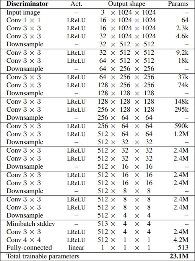
And at the end of this section let's create the discriminator\critic, I am not sure what to name it because the authors of WGAN-GP name it critic and we are using WGAN-GP.  But it's just a name, the point is to understand it and implement it right.  

In the figure below you can notice that the generator and discriminator are roughly mirrored images of each other, and always grow in synchrony.

• In the init part we send in_channels and im_channels, and we initialize leaky by LeakyReLu with the slide of 0.2,  prog_blocks (remember they are going to be in opposite ordering, we downsample instead of upsampling) by ModuleList() that will contain all the progressive blocks, rgb_blocks by ModuleList() that will contain all the RGB blocks, initial_rgb by WSConv2d that maps img_channels(3 for RGB) to in_channels, avg_pool for downsampling and final black which is the only different pattern from others (see the figure above).
• In the fade_in part, we send alpha, downscaled from the average pooling, out from the conv layer, and we return  [alpha * out + (1 - alpha) * downscaled]
• For Minibatch std on Discriminator, we add the minibatch_std part when we take the std for each example (across all channels, and pixels) then we repeat it for a single channel and concatenate it with the image. In this way, the discriminator will get information about the variation in the batch/image.
• In the forward part, we send x, the alpha value, and steps, and it going to be exactly the opposite of the forward part in the generator. In the initial step, we convert the image from RGB to in_channels depending on the image size, we check if steps=0 if it is we just use minibatch_std  and the final block, otherwise, we fade_in between downscaled and out, then we run through the progressive block that corresponds to the resolution of 'out', we downsample and we repeat that until we reach the resolution that we want depending on the steps, then we run it through minibatch_std and at the end we return the final_block.

class Discriminator(nn.Module):
    def __init__(self, in_channels, img_channels=3):
        super(Discriminator, self).__init__()
        self.prog_blocks, self.rgb_layers = nn.ModuleList([]), nn.ModuleList([])
        self.leaky = nn.LeakyReLU(0.2)

        # here we work back ways from factors because the discriminator
        # should be mirrored from the generator. So the first prog_block and
        # rgb layer we append will work for input size 1024x1024, then 512->256-> etc
        for i in range(len(factors) - 1, 0, -1):
            conv_in = int(in_channels * factors[i])
            conv_out = int(in_channels * factors[i - 1])
            self.prog_blocks.append(ConvBlock(conv_in, conv_out, use_pixelnorm=False))
            self.rgb_layers.append(
                WSConv2d(img_channels, conv_in, kernel_size=1, stride=1, padding=0)
            )

        # perhaps confusing name "initial_rgb" this is just the RGB layer for 4x4 input size
        # did this to "mirror" the generator initial_rgb
        self.initial_rgb = WSConv2d(
            img_channels, in_channels, kernel_size=1, stride=1, padding=0
        )
        self.rgb_layers.append(self.initial_rgb)
        self.avg_pool = nn.AvgPool2d(
            kernel_size=2, stride=2
        )  # down sampling using avg pool

        # this is the block for 4x4 input size
        self.final_block = nn.Sequential(
            # +1 to in_channels because we concatenate from MiniBatch std
            WSConv2d(in_channels + 1, in_channels, kernel_size=3, padding=1),
            nn.LeakyReLU(0.2),
            WSConv2d(in_channels, in_channels, kernel_size=4, padding=0, stride=1),
            nn.LeakyReLU(0.2),
            WSConv2d(
                in_channels, 1, kernel_size=1, padding=0, stride=1
            ),  # we use this instead of linear layer
        )

    def fade_in(self, alpha, downscaled, out):
        """Used to fade in downscaled using avg pooling and output from CNN"""
        # alpha should be scalar within [0, 1], and upscale.shape == generated.shape
        return alpha * out + (1 - alpha) * downscaled

    def minibatch_std(self, x):
        batch_statistics = (
            torch.std(x, dim=0).mean().repeat(x.shape[0], 1, x.shape[2], x.shape[3])
        )
        # we take the std for each example (across all channels, and pixels) then we repeat it
        # for a single channel and concatenate it with the image. In this way the discriminator
        # will get information about the variation in the batch/image
        return torch.cat([x, batch_statistics], dim=1)

    def forward(self, x, alpha, steps):
        # where we should start in the list of prog_blocks, maybe a bit confusing but
        # the last is for the 4x4. So example let's say steps=1, then we should start
        # at the second to last because input_size will be 8x8. If steps==0 we just
        # use the final block
        cur_step = len(self.prog_blocks) - steps

        # convert from rgb as initial step, this will depend on
        # the image size (each will have it's on rgb layer)
        out = self.leaky(self.rgb_layers[cur_step](x))

        if steps == 0:  # i.e, image is 4x4
            out = self.minibatch_std(out)
            return self.final_block(out).view(out.shape[0], -1)

        # because prog_blocks might change the channels, for down scale we use rgb_layer
        # from previous/smaller size which in our case correlates to +1 in the indexing
        downscaled = self.leaky(self.rgb_layers[cur_step + 1](self.avg_pool(x)))
        out = self.avg_pool(self.prog_blocks[cur_step](out))

        # the fade_in is done first between the downscaled and the input
        # this is opposite from the generator
        out = self.fade_in(alpha, downscaled, out)

        for step in range(cur_step + 1, len(self.prog_blocks)):
            out = self.prog_blocks[step](out)
            out = self.avg_pool(out)

        out = self.minibatch_std(out)
        return self.final_block(out).view(out.shape[0], -1)

Utils

In the code snippet below you can find the gradient_penalty function for WGAN-GP loss.

def gradient_penalty(critic, real, fake, alpha, train_step, device="cpu"):
    BATCH_SIZE, C, H, W = real.shape
    beta = torch.rand((BATCH_SIZE, 1, 1, 1)).repeat(1, C, H, W).to(device)
    interpolated_images = real * beta + fake.detach() * (1 - beta)
    interpolated_images.requires_grad_(True)

    # Calculate critic scores
    mixed_scores = critic(interpolated_images, alpha, train_step)
 
    # Take the gradient of the scores with respect to the images
    gradient = torch.autograd.grad(
        inputs=interpolated_images,
        outputs=mixed_scores,
        grad_outputs=torch.ones_like(mixed_scores),
        create_graph=True,
        retain_graph=True,
    )[0]
    gradient = gradient.view(gradient.shape[0], -1)
    gradient_norm = gradient.norm(2, dim=1)
    gradient_penalty = torch.mean((gradient_norm - 1) ** 2)
    return gradient_penalty

In the code snippet below you can find the generate_examples function that takes the generator gen, the number of steps to identify the current resolution, and a number n=100. The goal of this function is to generate n fake images and save them as a result.

def generate_examples(gen, steps, n=100):

    gen.eval()
    alpha = 1.0
    for i in range(n):
        with torch.no_grad():
            noise = torch.randn(1, Z_DIM, 1, 1).to(DEVICE)
            img = gen(noise, alpha, steps)
            if not os.path.exists(f'saved_examples/step{steps}'):
                os.makedirs(f'saved_examples/step{steps}')
            save_image(img*0.5+0.5, f"saved_examples/step{steps}/img_{i}.png")
    gen.train()

Training

In this section, we will train our ProGAN

First, let's use this line of code to give us some additional performance benefits.

torch.backends.cudnn.benchmarks = True

Train function

First, we loop over all the mini-batch sizes that we create with the DataLoader, and we take just the images because we don't need a label, then we identify the current batch size because we need it later.

Then we set up the training for the discriminator\Critic when we want to maximize E(critic(real)) - E(critic(fake)). This equation means how much the critic can distinguish between real and fake images if we have a large value that means the difference between them is large, if the value is null that means the critic can't distinguish between them at all.

After that, we set up the training for the generator when we want to maximize E(critic(fake)). Because the generator wants to fool the critic, so maximizing this equation means making this E(critic(real)) - E(critic(fake)) a smaller value, which is the opposite of what the critic want.

Finally, we update the alpha value for fade_in and ensure that it is between 0 and 1, and we return it.

def train_fn(
    critic,
    gen,
    loader,
    dataset,
    step,
    alpha,
    opt_critic,
    opt_gen,
):
    loop = tqdm(loader, leave=True)
    for batch_idx, (real, _) in enumerate(loop):
        real = real.to(DEVICE)
        cur_batch_size = real.shape[0]

        # Train Critic: max E[critic(real)] - E[critic(fake)] <-> min -E[critic(real)] + E[critic(fake)]
        # which is equivalent to minimizing the negative of the expression
        noise = torch.randn(cur_batch_size, Z_DIM, 1, 1).to(DEVICE)

        fake = gen(noise, alpha, step)
        critic_real = critic(real, alpha, step)
        critic_fake = critic(fake.detach(), alpha, step)
        gp = gradient_penalty(critic, real, fake, alpha, step, device=DEVICE)
        loss_critic = (
            -(torch.mean(critic_real) - torch.mean(critic_fake))
            + LAMBDA_GP * gp
            + (0.001 * torch.mean(critic_real ** 2))
        )

        critic.zero_grad()
        loss_critic.backward()
        opt_critic.step()

        # Train Generator: max E[critic(gen_fake)] <-> min -E[critic(gen_fake)]
        gen_fake = critic(fake, alpha, step)
        loss_gen = -torch.mean(gen_fake)

        gen.zero_grad()
        loss_gen.backward()
        opt_gen.step()

        # Update alpha and ensure less than 1
        alpha += cur_batch_size / (
            (PROGRESSIVE_EPOCHS[step] * 0.5) * len(dataset)
        )
        alpha = min(alpha, 1)

        loop.set_postfix(
            gp=gp.item(),
            loss_critic=loss_critic.item(),
        )
        

    return alpha

Training

Now since we have everything let's put them together to train our ProGAN.

We start by initializing the generator, the discriminator/critic, and optimizers in the same way that they did in the paper, then convert the generator and the critic into train mode, then loop over PROGRESSIVE_EPOCHS, and in each loop, we train the model number of epoch times, then we generate some fake images and save them, as a result, using generate_examples function, and finally, we progress to the next image resolution.

# initialize gen and disc, note: discriminator we called critic,
# according to WGAN paper (since it no longer outputs between [0, 1])
gen = Generator(
    Z_DIM, IN_CHANNELS, img_channels=CHANNELS_IMG
).to(DEVICE)
critic = Discriminator(
    IN_CHANNELS, img_channels=CHANNELS_IMG
).to(DEVICE)

# initialize optimizers
opt_gen = optim.Adam(gen.parameters(), lr=LEARNING_RATE, betas=(0.0, 0.99))
opt_critic = optim.Adam(
    critic.parameters(), lr=LEARNING_RATE, betas=(0.0, 0.99)
)


gen.train()
critic.train()

step = int(log2(START_TRAIN_AT_IMG_SIZE / 4))
for num_epochs in PROGRESSIVE_EPOCHS:
    alpha = 1e-5  # start with very low alpha, you can start with alpha=0
    loader, dataset = get_loader(4 * 2 ** step)  # 4->0, 8->1, 16->2, 32->3, 64 -> 4
    print(f"Current image size: {4 * 2 ** step}")

    for epoch in range(num_epochs):
        print(f"Epoch [{epoch+1}/{num_epochs}]")
        alpha = train_fn(
            critic,
            gen,
            loader,
            dataset,
            step,
            alpha,
            opt_critic,
            opt_gen,
        )
    generate_examples(gen, step, n=100)


    step += 1  # progress to the next img size

Result

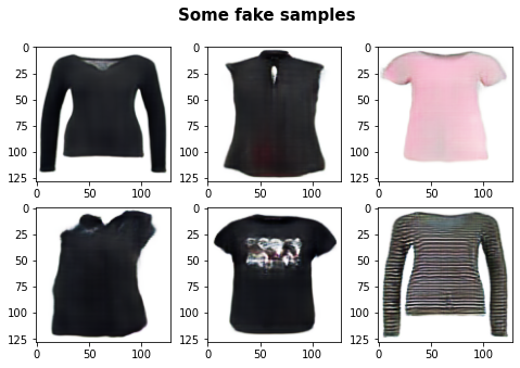
In the figure below you can see the result that we obtain after training this ProGAN in this dataset with 128*x 128 resolution.

Conclusion

In this article, we make a clean, simple, and readable implementation from scratch of ProGAN with the key attributions from the paper (Progressive growing, Fading in new layers, Minibatch std on Discriminator, Normalization with PixelNorm, and Equalized Learning Rate) using PyTorch.

In the upcoming articles, we will explain in depth and implement from scratch StyleGANs to generate also some cool fashion.