Getting Started With DCGANs

The development of Generative Adversarial Networks (GANS) is a revolutionary achievement. While there have been many breakthrough advancements for developers in the field of deep learning, none of the results produced by the previous generative methodologies were satisfactory. GANs became the first method to achieve convincingly high-quality results on most datasets that they were tested with. Since 2014, GANs have remained as one of the most popular aspects of study in neural networks and deep learning. In my previous article on "Complete Guide to Generative Adversarial Networks (GANs)," which you can access from the following link, we covered most of the essential concepts required for the basic understanding of GANs. These included topics such as generative and discriminative models, types of generative models, in-depth understanding of their training procedure, and their applications in the modern world.

With the rise in popularity of these Generative Adversarial Networks, we have many variations of GANs, including DCGANs, SRGAN, Pix2Pix, Cycle GAN, ProGAN, and so much more. While we will look at other GAN archetypes in future articles, our focus for this section will be on Deep Convolutional Generative Adversarial Networks (DCGANs). In this article, we will introduce ourselves to DCGANs and dwell slightly deeper into some of their intricate aspects. Then, we will construct a project from scratch by using these DCGANs for number generation. The table of contents provided below will guide you through the various sections of this article. Although it is recommended to check out each individual aspect in further detail, you can feel free to skip ahead to the sections that intrigue you the most.

Introduction:

While the popularity of GANs is now peaking with immense success, the situation and love for this concept were not always as special as one would now expect. The redeeming qualities of GANs were the lack of a heuristic cost function (a good example is the pixel-wise independent mean square loss) and the fact that it was one of the better methods of generative models. However, there was a lack of computation requirements, innovative ideas, and the noticeable fact that GANs mostly generated non-sensical results. Due to these reasons, Convolutional Neural Networks (CNNs) were primarily used for constructing tasks related to supervised learning, such as classification problems, because these complications could easily be achieved and solved with the help of CNN's.

In the modern era, CNNs are not limited to supervised classification problems. With the introduction of DCGANs, we noticed that CNNs had an increasingly high potential for producing high-quality results on numerous tasks. With DCGANs, the successful accomplishment of unsupervised tasks and generative models was made possible. For the DCGANs architecture, we will reference the popular "Unsupervised Representation Learning with Deep Convolutional Generative Adversarial Networks" research paper, which covers this topic extensively. The primary objective of the DCGANs architecture is to set up the initial parameters for evaluation of a set of constraints to always achieve stable testing results in most settings and technical scenarios. Once the primary model is constructed, the discriminator serves the purpose of showing a highly competitive performance for image classification tasks on par with other popular unsupervised learning algorithms.

Once the discriminator is completely trained, we can utilize this model to classify the generated images from the generator as real or fake. The generator model's objective is to generate an image so realistic that it can bypass the testing process of classification from the discriminator. The generator model developed in the DCGANs archetype has intriguing vector arithmetic properties, which allows for the manipulation of many semantic qualities of generated samples. With this basic introduction to DCGANs and all of their initial features, let us look at their architecture in the next section of this article.

Dwelling deeper into DCGANs Architecture:

As discussed previously, convolutional neural networks were more successful on supervised tasks related to classification or other similar problems. With the introduction of the DCGANs research paper, this thinking approach changed as the architecture developed produced highly desirable results on a large scale of data enabling it to even process higher resolution images. Due to this successful method of implementation on many significant datasets, it becomes essential to understand the core concepts utilized to make the involvement of CNN in GANs make it perform exceptionally.

The few conceptual ideas of implementation include the use of convolutional networks with striding replacing the max-pooling structure. This structure allows the generator model to learn its own spatial dimensions with the help of upsampling through Conv2D transpose while simultaneously using the striding operation for allowing the network to also learn its respective downsampling. The first layer of the DCGAN takes a uniformly distributed value labeled $Z$. The input layer is perhaps the only layer that utilizes Dense layers. Apart from this exception, none of the other layers use either fully connected or max-pooling layers.

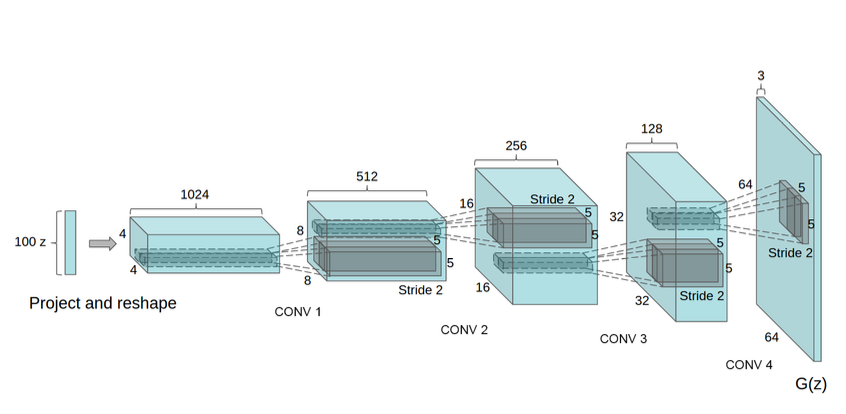
From the above image representation, we can understand that there is a 100-dimensional uniformly distributed noise labeled $Z$ for the LSUN dataset. This dimensionality is projected on a smaller spatial extension containing a convolutional representation with many feature maps. The architecture described in the above image is followed by a series of four blocks of fractionally-strided convolutions, which help to contribute to the previously discussed spatial dimensional learning of the model. The random noise initialized at the beginning will eventually learn the prominent features with the help of continuous upsampling through the fractionally-strided convolutions.

The other critical aspects involved in the designing of the model include the use of batch normalization layers. These batch normalization layers are extensively used in both the generator and discriminator models for obtaining the stability of the model. Research shows that by applying the batch normalization process, most of the training issues that arise due to the initialization of the inputs are solved. It also helps for better gradient flow in the layers by normalizing the input to each unit to have zero mean and unit variance. Finally, all the layers will be followed by the ReLU activation functions in the generator models except the output layer, which contains the tanh activation function. All the layers in the discriminator model will contain the Leaky ReLU activation function as they are shown to produce the best results.

Number Generation With DCGANs:

For understanding the working of DCGANs from scratch, we will construct a project on number generation with DCGANs with the help of the MNIST dataset. The MNIST data stands for Modified National Institute of Standards and Technology database, which is one of the most popular datasets encompassing a large-scale availability of 60,000 examples on the training dataset, and a test set consisting of 10,000 examples. It is often a great starting point for anyone interested in testing any kind of network. We will use the generator and discriminator models of the DCGANs to learn from this dataset. Once the training is complete, we will use the generator model to hopefully generate some decently high-quality results.

For the completion of this project, we will utilize the TensorFlow and Keras deep learning frameworks. If you don't have complete knowledge of these two libraries or want to quickly refresh your basics, I would recommend checking out the following link for TensorFlow and this particular link for Keras. Ensure that you have sufficient knowledge moving further. The first step in our project is to import all the essential libraries. We will use matplotlib for visualizing our data, the numpy library for accessing the images in the form of arrays, the TensorFlow and Keras deep learning frameworks for constructing the DCGANs architecture, and other libraries for their specific use cases.

The most significant import is the MNIST dataset which is available to us pre-built in the core TensorFlow and Keras library. We will access this dataset directly from the frameworks rather than performing an external installation. The code for all the required imports is provided below.

Importing The Required Libraries:

import matplotlib.pyplot as plt
import tensorflow as tf
import numpy as np
import PIL 
import glob
from tensorflow.keras.datasets.mnist import load_data 
from tensorflow.keras.layers import Conv2D, Dense, Flatten, MaxPooling2D, BatchNormalization, Dropout, LeakyReLU
from tensorflow.keras.layers import Conv2DTranspose, Reshape
from tensorflow.keras.models import Sequential, Model
from tensorflow.keras.optimizers import Adam
import time
import imageio
from IPython import display
import os

Load The Data:

Now that we have imported all the required libraries for the number generation project, let us load the data. Since the MNIST dataset is divided into images and their respective labels separately for both the training and testing data, we can use the code block below to load the appropriate data accordingly. Due to the direct import of the MNIST dataset from the Keras library, this action can be performed with relative ease.

(train_images, train_labels),(test_images, test_labels) = load_data()

Visualizing our data:

The next step we will perform is the visualization of the dataset. We will visualize the first twenty-five elements of the data with the help of the matplotlib library. We will plot these elements and ensure that they are mapped to the binary element composition. The binary mapping means these images are viewed as grayscale images. Each image provided in the MNIST dataset has the parameters of $28 × 28 × 1$ array of floating-point numbers for representing the grayscale intensities which range from values of $0$ (black) to $1$ (white). The dimensions are of width and height of $28 × 28$, and the channel length is $1$ for grayscale images. The code below plots the appropriate data accordingly.

for i in range(25):
    plt.subplot(5, 5, 1 + i)
    plt.axis("off")
    plt.imshow(train_images[i], cmap=plt.cm.binary)
    
plt.show()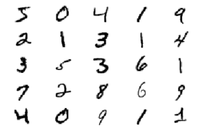

If you want to visualize a single image without using any cmap function, you can do so with the following line of code.

plt.imshow(train_images[0])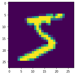

Setting Parameters:

Our next step will be to normalize the dataset accordingly and set some of the initial parameters for the particular task of number generation. Firstly, we will reshape our training images in a format that is suitable for passing them through the convolutional neural networks in the DCGANs architecture. We will convert all of the data to floating type variables and normalize the data. The normalization procedure ensures that all the data provided in the dataset is in a range of $0$ to $1$ rather than $0$ to $255$. Doing so will ensure that the computation of the task is slightly faster and more efficient. We will also set the buffer size and batch size accordingly. The buffer size will be set as $60000$, which is equivalent to the number of training examples. The batch size can be set according to the convenience and limitations of your hardware. We will use the tensor slices to shuffle the training dataset according to the pre-set parameters.

# Normalize The Training images accordingly

train_images = train_images.reshape(train_images.shape[0], 28, 28, 1).astype('float32')
train_images = (train_images - 127.5) / 127.5  

BUFFER_SIZE = 60000
BATCH_SIZE = 256

# Batch and shuffle the data
train_dataset = tf.data.Dataset.from_tensor_slices(train_images).shuffle(BUFFER_SIZE).batch(BATCH_SIZE)

After performing all the initial steps required for the project of number generation from scratch, including importing the essential libraries, loading the appropriate data, visualizing the data, and setting the initial parameters, we can proceed to the next steps of the article. In the next section, we will explore how to construct the generator and discriminator models for the following project as described in the research paper.

Building the generator and discriminator models:

For constructing the generator and discriminator models, we will utilize the TensorFlow and Keras deep learning frameworks as previously discussed. We will also make use of the official TensorFlow generative model section as a reference for building both our architectures. Most of the core designing process for the DCGANs architectural structure remains the same as discussed in the previous section of the DCGANs architecture. There are a few slight noticeable changes that we will discuss accordingly. Let us get started with the construction of the generator and discriminator models.

Generator:

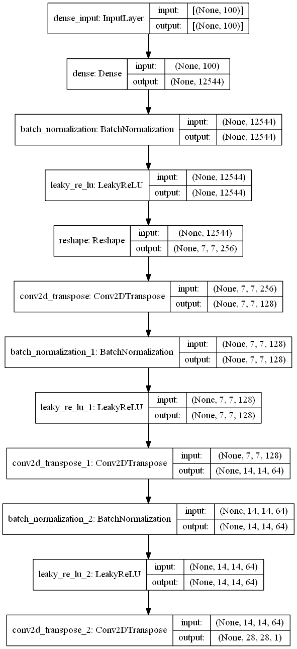
We will now construct the generator architecture with a Sequential model style. We will define the initial model with an input shape of 100 for receiving the incoming random noise seed, which will be passed through further layers of convolutional upsampling with striding layers. As discussed in the DCGANs architecture, the generator model is composed of mostly convolutional upsampling layers with strides. There are no max-pooling layers used in the architecture.

Each layer is followed by a batch normalization layer for stability and faster gradient initializations. However, the slightly noticeable change is the use of Leaky ReLU layers over the ReLU activation function, as mentioned in the research paper. You can explore these factors accordingly to see which method produces the best results. Regardless, the difference for either method should not be greatly variable. The final layer uses the tanh activation, as mentioned in the research paper. The objective of the generator is to upsample its spatial dimensions until it reaches the desired image size of $28 x 28 x 1$.

def The_Generator():
    model = Sequential()
    
    model.add(Dense(7*7*256, use_bias=False, input_shape=(100,)))
    model.add(BatchNormalization())
    model.add(LeakyReLU())
      
    model.add(Reshape((7, 7, 256)))
    assert model.output_shape == (None, 7, 7, 256) # Note: None is the batch size
    
    model.add(Conv2DTranspose(128, (5, 5), strides=(1, 1), padding='same', use_bias=False))
    assert model.output_shape == (None, 7, 7, 128)  
    model.add(BatchNormalization())
    model.add(LeakyReLU())

    model.add(Conv2DTranspose(64, (5, 5), strides=(2, 2), padding='same', use_bias=False))
    assert model.output_shape == (None, 14, 14, 64)    
    model.add(BatchNormalization())
    model.add(LeakyReLU())

    model.add(Conv2DTranspose(1, (5, 5), strides=(2, 2), padding='same', use_bias=False, activation='tanh'))
    assert model.output_shape == (None, 28, 28, 1)
  
    return model
    
generator = The_Generator()

We will store the generator model in the "generator" variable. Let us explore the model summary and the model plot produced by this generator model. Doing so will help us to conceptually understand the type of model architecture built and perform further analysis on the same.

Model Summary:

Model: "sequential"
_________________________________________________________________
Layer (type)                 Output Shape              Param #   
=================================================================
dense (Dense)                (None, 12544)             1254400   
_________________________________________________________________
batch_normalization (BatchNo (None, 12544)             50176     
_________________________________________________________________
leaky_re_lu (LeakyReLU)      (None, 12544)             0         
_________________________________________________________________
reshape (Reshape)            (None, 7, 7, 256)         0         
_________________________________________________________________
conv2d_transpose (Conv2DTran (None, 7, 7, 128)         819200    
_________________________________________________________________
batch_normalization_1 (Batch (None, 7, 7, 128)         512       
_________________________________________________________________
leaky_re_lu_1 (LeakyReLU)    (None, 7, 7, 128)         0         
_________________________________________________________________
conv2d_transpose_1 (Conv2DTr (None, 14, 14, 64)        204800    
_________________________________________________________________
batch_normalization_2 (Batch (None, 14, 14, 64)        256       
_________________________________________________________________
leaky_re_lu_2 (LeakyReLU)    (None, 14, 14, 64)        0         
_________________________________________________________________
conv2d_transpose_2 (Conv2DTr (None, 28, 28, 1)         1600      
=================================================================
Total params: 2,330,944
Trainable params: 2,305,472
Non-trainable params: 25,472
_________________________________________________________________

Model Plot:

Random Visualizations for generator images:

Now that we have built the model and analyzed the plot and summary, let us also visualize the kind of output that an untrained generator would produce with a random noise distribution. We will pass the random noise through the generator and obtain a result, i.e., a generated image from the generator.

# Visualizing the random image generated by the generator

noise = tf.random.normal([1, 100])
generated_image = generator(noise, training=False)

plt.imshow(generated_image[0, :, :, 0])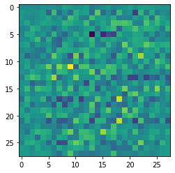

The above image is a representation of the color image type of output that would normally be produced. However, we know that our MNIST data consists of grayscale images. Hence, let us try to visualize the generated output with the parameters set for grayscale images.

plt.imshow(generated_image[0, :, :, 0], cmap='gray')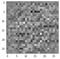

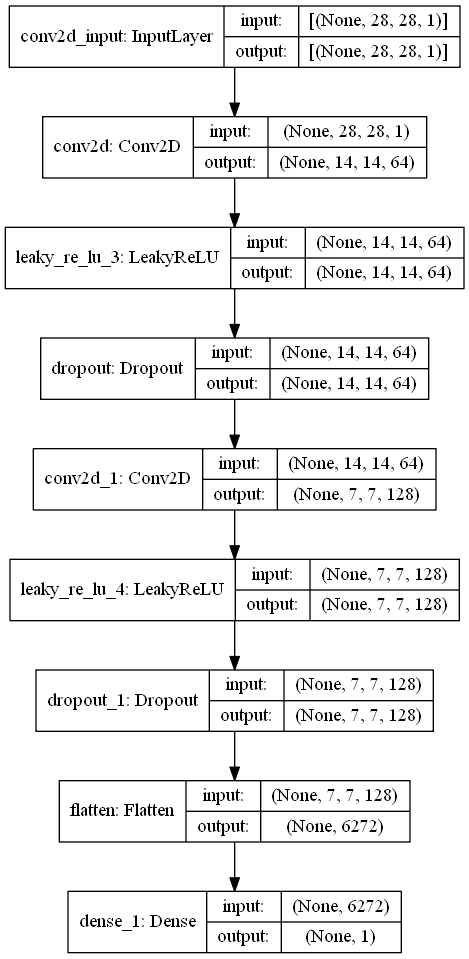
Discriminator:

Now that we have a brief idea of the working procedure of the generator and the type of outputs they produce, we can proceed to construct the discriminator model for the DCGANs architecture as well. We will use the Sequential model architecture type for the discriminator too similar to the generator. We will use convolutional layers followed by the Leaky ReLU activation functions as described in the research paper. However, we also add an additional layer to prevent over-fitting and obtain better classification results through the use of dropout. Finally, we will flatten the architecture and use a final dense layer containing one node to make the appropriate predictions. The prediction by the discriminator output positive values for real images and negative values for fake images.

def The_Discriminator():
    model = Sequential()
    
    model.add(Conv2D(64, (5, 5), strides=(2, 2), padding='same', input_shape=[28, 28, 1]))
    model.add(LeakyReLU())
    model.add(Dropout(0.3))
      
    model.add(Conv2D(128, (5, 5), strides=(2, 2), padding='same'))
    model.add(LeakyReLU())
    model.add(Dropout(0.3))
       
    model.add(Flatten())
    model.add(Dense(1))
     
    return model
    
discriminator = The_Discriminator()

Let us explore the model summary and the model plot of the discriminator to help us understand how the architecture looks visually.

Model Summary:

Model: "sequential_1"
_________________________________________________________________
Layer (type)                 Output Shape              Param #   
=================================================================
conv2d (Conv2D)              (None, 14, 14, 64)        1664      
_________________________________________________________________
leaky_re_lu_3 (LeakyReLU)    (None, 14, 14, 64)        0         
_________________________________________________________________
dropout (Dropout)            (None, 14, 14, 64)        0         
_________________________________________________________________
conv2d_1 (Conv2D)            (None, 7, 7, 128)         204928    
_________________________________________________________________
leaky_re_lu_4 (LeakyReLU)    (None, 7, 7, 128)         0         
_________________________________________________________________
dropout_1 (Dropout)          (None, 7, 7, 128)         0         
_________________________________________________________________
flatten (Flatten)            (None, 6272)              0         
_________________________________________________________________
dense_1 (Dense)              (None, 1)                 6273      
=================================================================
Total params: 212,865
Trainable params: 212,865
Non-trainable params: 0
_________________________________________________________________

Model Plot:

Making a decision:

The objective of the discriminator is to classify if the image output produces a real or fake image. Let us see the type of output a single decision of the discriminator provides us. Note that the model is trained such that positive values imply that the image is real, while a negative value implies the image is fake.

decision = discriminator(generated_image)
print(decision)

Output:

tf.Tensor([[0.0015949]], shape=(1, 1), dtype=float32) 

Now that we have constructed both the generator and discriminator architecture models, we can proceed to build the entire DCGANs model together and train the parameters accordingly to achieve the best possible results.

Constructing the DCGANs Model:

After the completion of all the initial pre-processing steps and construction of the generator and discriminator models individually, we can proceed to build the entire DCGANs model and train it accordingly to achieve the best results possible. This section of the article is divided into four crucial steps for the perfect working of the model. We will first define the loss and optimizer that we will utilize for the compilation of the model. After this, we will create a checkpoint so that we can reuse the model when required. We will then define all the essential parameters and set the @tf function, which will automatically compile the model. Finally, we will train the model and proceed to visualize the generated images by the DCGANs model. Let us get started by defining the loss parameter and the optimizer.

Define the loss and optimizers:

The next significant step we will perform for the construction of the DCGANs model is defining the loss functions and initializing the optimizers. We will define our loss function, which will take in the output parameters as binary cross-entropy. We will set the logits attribute as true. The logit attribute informs the loss function that the output values generated by the model are not normalized. Doing so is helpful because we know that the job of the discriminator is to classify the output. Hence, negative values represent fake and positive values represent the real image. After the definition of the discriminator and generator losses, we will define the optimizers for both of them as well. We will use the Adam optimizers for both these models. Let us explore the code block and then try to further understand intuitively what they do.

cross_entropy = tf.keras.losses.BinaryCrossentropy(from_logits=True)

def discriminator_loss(real_output, fake_output):
    real_loss = cross_entropy(tf.ones_like(real_output), real_output)
    fake_loss = cross_entropy(tf.zeros_like(fake_output), fake_output)
    total_loss = real_loss + fake_loss
    return total_loss

def generator_loss(fake_output):
    return cross_entropy(tf.ones_like(fake_output), fake_output)
    
generator_optimizer = tf.keras.optimizers.Adam(1e-4)
discriminator_optimizer = tf.keras.optimizers.Adam(1e-4)

In the above code block, the real output refers to all the real labels from the original dataset, whereas the fake output refers to all the generated labels from the generator model outputs. The total loss generated from the following code block will result in the following equation:

$$total  loss = -log(real  output) - log(1 - fake  output)$$

The above equation for the discriminator tries to minimize the loss function for obtaining better results.

Define the checkpoint:

With an average GPU, GANs take quite some time to train. We will define checkpoints so that if we want to re-train the model again after a specific set of epochs, we can restore the checkpoints to continue our training.

checkpoint_dir = './training_checkpoints'
checkpoint_prefix = os.path.join(checkpoint_dir, "ckpt")
checkpoint = tf.train.Checkpoint(generator_optimizer=generator_optimizer,
                                 discriminator_optimizer=discriminator_optimizer,
                                 generator=generator,
                                 discriminator=discriminator)

Set the essential parameters and define @tf.function:

In the next step, we will define some essential parameters. We will reuse the seed that we defined so that it becomes easier for us to visualize the overall progress of the generated animated GIF over time. I will run the model for a total of 100 epochs. You can choose to do more or less according to your requirements and system limitations.

EPOCHS = 100
noise_dim = 100
num_examples_to_generate = 16

seed = tf.random.normal([num_examples_to_generate, noise_dim])

Our next step is to define the @tf.function that causes the model to be compiled. We will make use of the of the GradientTape() function available to us in TensorFlow to manually start training both the generator and discriminator models. The task of the generator is to generate images so good that it can bypass the discriminator. The task of the discriminator is to distinguish the real and fake images accordingly. Once the generator generates top-notch results to bypass the discriminator's classification system, we have built a high-quality DCGANs model to successfully complete the particular task.

@tf.function
def train_step(images):
    noise = tf.random.normal([BATCH_SIZE, noise_dim])

    with tf.GradientTape() as gen_tape, tf.GradientTape() as disc_tape:
        generated_images = generator(noise, training=True)

        real_output = discriminator(images, training=True)
        fake_output = discriminator(generated_images, training=True)

        gen_loss = generator_loss(fake_output)
        disc_loss = discriminator_loss(real_output, fake_output)

    gradients_of_generator = gen_tape.gradient(gen_loss, generator.trainable_variables)
    gradients_of_discriminator = disc_tape.gradient(disc_loss, discriminator.trainable_variables)

    generator_optimizer.apply_gradients(zip(gradients_of_generator, generator.trainable_variables))
    discriminator_optimizer.apply_gradients(zip(gradients_of_discriminator, discriminator.trainable_variables))

Training and generating the images:

With all the other steps completed, we can finally begin the training process. We will now define the training function that will utilize all the functions that we previously defined for our model. We will also print the take the time taken to run each individual epoch and the type of image generated from the start. Doing so will help us to see the learning curve of our model visually and gain a better understanding of the training process.

def train(dataset, epochs):
    for epoch in range(epochs):
        start = time.time()

        for image_batch in dataset:
            train_step(image_batch)

        # Produce the images for the GIF with each step
        display.clear_output(wait=True)
        generate_and_save_images(generator,
                                 epoch + 1,
                                 seed)

        # Save the model every 15 epochs
        if (epoch + 1) % 15 == 0:
            checkpoint.save(file_prefix = checkpoint_prefix)

        print ('Time for epoch {} is {} sec'.format(epoch + 1, time.time()-start))

    # Generate after the final epoch
    display.clear_output(wait=True)
    generate_and_save_images(generator,
                           epochs,
                           seed)

You can use the following code block from our TensorFlow reference for generating and saving the images that are generated in each epoch.

def generate_and_save_images(model, epoch, test_input):
    # Notice `training` is set to False.
    # This is so all layers run in inference mode (batchnorm).
    predictions = model(test_input, training=False)

    fig = plt.figure(figsize=(4, 4))

    for i in range(predictions.shape[0]):
        plt.subplot(4, 4, i+1)
        plt.imshow(predictions[i, :, :, 0] * 127.5 + 127.5, cmap='gray')
        plt.axis('off')

    plt.savefig('image_at_epoch_{:04d}.png'.format(epoch))
    plt.show()

Now that we have completed all the primary steps, let us call the function that will start training the model. Once the training is completed, we can start visualizing the outputs produced.

train(train_dataset, EPOCHS)

The above image representation is a screenshot after 100 epochs of training. The entire notebook for this project is attached to the article. Feel free to explore it accordingly.

Conclusion:

The abilities of Generative Adversarial Networks to generate fake visuals, images, text, or other entities with some random noise are complementary. One variation of GANs, which is the Deep Convolutional Generative Adversarial Networks (DCGANs), produces fantastic results on some of the datasets in which it is tested. From our previous knowledge of GANs from this article and our understanding of DCGANs from this article, we can construct lots of fabulous projects with deep learning frameworks such as TensorFlow, Keras, and PyTorch.

In this article, we briefly understood the working procedure of DCGANs and the various techniques employed in the "Unsupervised Representation Learning with Deep Convolutional Generative Adversarial Networks" research paper. We then worked on the project of number generation with the help of the MNIST dataset. Using this dataset, we pre-processed the initial data and constructed the appropriate generator and discriminator models to train them. After training the data with the DCGANs architecture, we were able to generate pretty decent results after just fifty epochs of training. With further training and model improvements, it would be possible to achieve even better results on the datasets.

In the upcoming parts of the Generative Adversarial Networks, we will expand on the applications of DCGANs and look into how to construct a face generation project with images to produce realistic facial images of people who don't exist. We will also look into more GAN variations, projects, and topics in future articles. Until then, keep coding and exploring!