The technological advancements and developments in machine learning, deep learning, and neural networks have led to a revolutionary era. Creating and replicating photos, texts, images, and pictures based on only a collection of examples can be considered shocking to some, and marvelous to others.
We are now at a point where technology is so advanced that deep learning and neural networks can even generate realistic human faces from scratch. The faces generated do not belong to any person, alive or dead, yet they are astoundingly realistic.
One special deep learning network we have to thank for these achievements is the Generative Adversarial Network (GAN), which is the topic of this article. Let's briefly explore our table of contents to understand the main topics we'll cover.
Table of Contents
- Introduction to GANs
- Understanding Generative and Discriminative Models
- Types of Generative Models
1. Variational Autoencoders (VAE)
2. Generative Adversarial Networks (GANs) - Discriminators
- Generators
- In-depth Understanding of Training
- Applications
- Conclusion
Bring this project to life
Introduction to GANs
Generative Adversarial Networks (GANs) were developed in 2014 by Ian Goodfellow and his teammates. GANs are a unique type of deep neural network that can generate new data with similarities to the data it is trained on. GANs have two main blocks that compete against each other to produce visionary creations. In this article, we'll gain a detailed understanding of how GANs work.
The more intricate details of this competition between the two blocks, called the generator and discriminator, will be discussed in further detail in the later sections of this article. Firstly, let us get an understanding of the various real-life use cases that Generative Adversarial Networks (GANs) see in tech companies, highlighting their relevance today.
Adobe makes use of GANs for next-generation Photoshop. Google utilizes the power of GANs for both generation of text as well as images. IBM effectively uses GANs for data augmentation. Snapchat uses them for efficient image filters and Disney for super resolutions. GANs have numerous uses and pose many advantages in the world market today, and their demand should only increase in the coming years.
In this article, our main aim is to intuitively understand the concepts of Generative Adversarial Networks. Apart from covering the theoretical aspects of GANs, we will also consider PyTorch code for each of the generator and discriminator model constructions.
Understanding Generative and Discriminative Models
Discriminative models in machine learning and deep learning play the role of a classifier. They are typically used to distinguish between two classes or a set of labels. A few examples of these kinds of tasks include distinguishing a dog from a cat, differentiating between various dog breeds, or classifying various fruits (like apple, grapes, oranges, etc.).
The generative models, on the other hand, work differently than their discriminative counterparts. In a generative model, you consider random samples (typically noise) and generate new realistic images from this noise. To give an example, a generative model can learn from real images of dogs to then create its own fake–yet realistic–dog images. There are two main types of generative models that we will discuss further in the next section.
Types of Generative Models
Variational Autoencoders
There are two main types of generative models, namely variational autoencoders and generative adversarial networks (GANs). While our main focus in this article will remain on GANs, we will also briefly understand the working of variational autoencoders in this section.
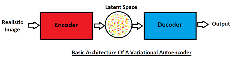
The variational autoencoder also makes use of encoders and decoders, which are usually independent neural networks. As shown in the above block diagram, a realistic image is passed through the encoder. The main function of the encoder is to represent these realistic images in the form of vectors in the latent space.
The decoder accepts these interpretations and produces copies of realistic images. Initially, the quality of the images produced might be low, but once the decoder is fully functional, the encoder can be completely disregarded. Some random noise samples can be introduced in the latent space, and realistic images will be generated by the decoder.
Generative Adversarial Networks
That brings us to the main focus of this article: GANs. Firstly, let's gain an intuitive understanding of GANs and understand exactly how these deep learning algorithms work.
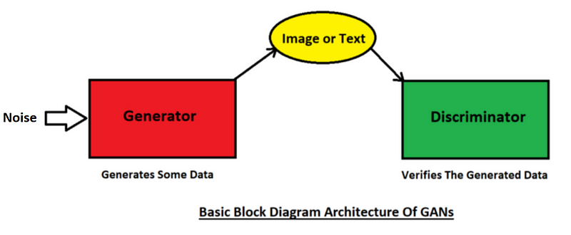
The generator and discriminator in a GAN compete against each other (hence the term "adversarial"). The generator is like a thief whose aim is to replicate and produce realistic data to trick the discriminator; the generator wants to bypass the numerous checks it will perform. On the other hand, the role of the discriminator is to act as the police and catch the artificially generated data as sold by the generator. The discriminator tries to catch the abnormalities and detect the false images made by the generator.
In other words, the generator takes in a noisy input and tries to produce realistic images from it. Even though it fails terribly at first, it slowly learns how to make more convincing counterfeits. The discriminator block then tries to determine which images are real and which ones are fake. So, these models compete against each other until a point of "perfection" is reached.
The point of perfection is said to be reached when the generator starts to generate multiple high-quality, realistic images and bypasses the testing phase of the discriminator. Once the images are successfully realistic, the discriminator cannot distinguish between the actual and fake images. After this point, you can use the generator on its own, and you don’t require a discriminator anymore.
Since we have already established that GANs consist mainly of these two building blocks, namely the generator and the discriminator, let us now look at them in further detail in the upcoming sections. In summary, these two blocks are separate neural networks:
- "Generators" are neural networks that learn to generate fake images (or data points) that look realistic, and can pass as real when fed to a discriminator network.
- "Discriminators" are neural networks that distinguish between real and fake images (or whatever type of data). The discriminator performs an essential role in the learning process of the generator.
Discriminators
The role of the discriminator is to distinguish between real and fake images. The discriminator basically acts as a classifier.
For example, let's consider a classifier that serves the role of identifying whether or not an image is of a dog (the classes essentially being: "Dog" and "Not Dog"). The classifier would give us a value between zero and one that indicates its confidence that the image is of a dog. The closer the value is to one, the higher the probability that the image is a dog, while a value closer to zero signifies the opposite.
For example: $P(Y|X) = 0.90$.
The $P(Y|X)$ format signifies a conditional probability, where the prediction of a label $Y$ is made given the features, $X$. The probability of $0.90$ in the above example indicates that the classifier is 90% confident that an image contains a dog. A similar pattern can be applied to discriminators to determine (or classify) an image as real or fake.
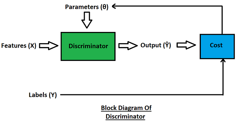
Moving forward to analyze the block diagram of the discriminator, we can briefly determine the methodology behind its working. The features ($X$) are passed through the discriminator, which acts as a classifier trying to make successful predictions on the features provided. The discriminator predicts an outcome ($Ŷ$) that is used for the calculation of the overall cost.
The procedure for the calculation of cost is quite simple as we determine the cost value (or the respective loss) by considering the predicted output ($Ŷ$ in this case) with the actual outcome values or labels ($Y$). After the successful computation of the cost function, we can update the respective parameters of the discriminator. We will discuss the exact working of these stages when we cover the training of the discriminator.
Let's look at some code for discriminators in PyTorch. This code is just a basic example, and can be altered as per the user’s choice. The code reference is taken from this course on building basic GANs. I highly recommend it to readers who are interested in building GANs themselves.
def get_discriminator_block(input_dim, output_dim):
    '''
    Discriminator Block
    Function for returning a neural network of the discriminator given input and output dimensions.
    Parameters:
        input_dim: the dimension of the input vector, a scalar
        output_dim: the dimension of the output vector, a scalar
    Returns:
        a discriminator neural network layer, with a linear transformation
          followed by an nn.LeakyReLU activation with negative slope of 0.2
          (https://pytorch.org/docs/master/generated/torch.nn.LeakyReLU.html)

    '''

    return nn.Sequential(
        nn.Linear(input_dim, output_dim),
        nn.LeakyReLU(0.2)
    )
class Discriminator(nn.Module):
    '''
    Discriminator Class
    Values:
        im_dim: the dimension of the images, fitted for the dataset used, a scalar
            (MNIST images are 28x28 = 784 so that is your default)
        hidden_dim: the inner dimension, a scalar

    '''

    def __init__(self, im_dim=784, hidden_dim=128):
        super(Discriminator, self).__init__()
        self.disc = nn.Sequential(
            get_discriminator_block(im_dim, hidden_dim * 4),
            get_discriminator_block(hidden_dim * 4, hidden_dim * 2),
            get_discriminator_block(hidden_dim * 2, hidden_dim),
            nn.Linear(hidden_dim, 1)
        )
def forward(self, image):
        '''
        Function for completing a forward pass of the discriminator: Given an image tensor,
        returns a 1-dimension tensor representing fake/real.
        Parameters:
            image: a flattened image tensor with dimension (im_dim)

        '''
        return self.disc(image)

    def get_disc(self):
        '''
        Returns:
            the sequential model
        '''
        return self.disc
Generators
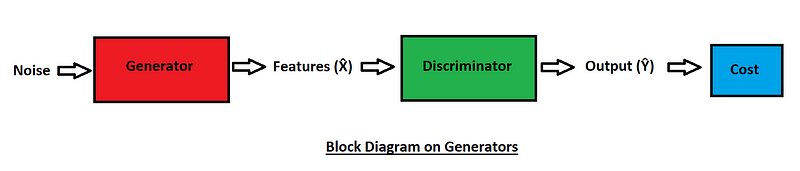
The role of the generator is to create fake images that look so realistic that it becomes impossible for the discriminator to distinguish between the real and fake images. Initially, the generator fails pretty badly at its job of generating realistic images due to the introduction of a random noise variable, and also because the generator has no idea what to generate. Over time, after the updating of its parameters, it can slowly learn patterns to bypass the discriminator.
From the block diagram shown in the above image, we can observe that the noise is passed through the generator neural network, which tries to produce a realistic output example. The generated output consists of a set of features $\hat{X}$ for the following generated image.
These features are fed to the discriminator, and it predicts or classifies how real or fake the current image produced by the generator is. The generator wants the output ($Ŷ$) to be as close to $1$ for a real image (here, $Ŷ$ refers to the predictions made by the discriminator). Using the difference between the actual output and the discriminator classifier output, we can compute the cost, where $1$ is for real images, while $0$ is for fake images.
The cost function calculated is used to update the parameters and improve the model. Once you can achieve a model that generates high-quality realistic images, you can save the parameters of the model. You can use this saved model by loading it and utilizing it for generating various outputs. Whenever new noise vectors are introduced, the generator will generate newer images for the trained data.
Let us look at some code for generators in PyTorch. These are just example code blocks, and can be altered as per the user’s choice. The code reference is taken from this course on building basic GANs. I would highly recommend it to readers who are interested in learning how to build GANs themselves.
def get_generator_block(input_dim, output_dim):
    '''
    Function for returning a block of the generator's neural network
    given input and output dimensions.
    Parameters:
        input_dim: the dimension of the input vector, a scalar
        output_dim: the dimension of the output vector, a scalar
    Returns:
        a generator neural network layer, with a linear transformation
          followed by a batch normalization and then a relu activation

    '''

    return nn.Sequential(
        nn.Linear(input_dim, output_dim),
        nn.BatchNorm1d(output_dim),
        nn.ReLU(inplace=True),
    )
class Generator(nn.Module):
    '''
    Generator Class
    Values:
        z_dim: the dimension of the noise vector, a scalar
        im_dim: the dimension of the images, fitted for the dataset used, a scalar
          (MNIST images are 28 x 28 = 784 so that is your default)
        hidden_dim: the inner dimension, a scalar

    '''

    def __init__(self, z_dim=10, im_dim=784, hidden_dim=128):
        super(Generator, self).__init__()
        # Build the neural network
        self.gen = nn.Sequential(
            get_generator_block(z_dim, hidden_dim),
            get_generator_block(hidden_dim, hidden_dim * 2),
            get_generator_block(hidden_dim * 2, hidden_dim * 4),
            get_generator_block(hidden_dim * 4, hidden_dim * 8),
            nn.Linear(hidden_dim * 8, im_dim),
            nn.Sigmoid()
        )

    def forward(self, noise):
        '''
        Function for completing a forward pass of the generator: Given a noise tensor,
        returns generated images.
        Parameters:
            noise: a noise tensor with dimensions (n_samples, z_dim)
        '''
        return self.gen(noise)

    def get_gen(self):
        '''
        Returns:
            the sequential model
        '''
        return self.gen
In-depth Understanding of Training
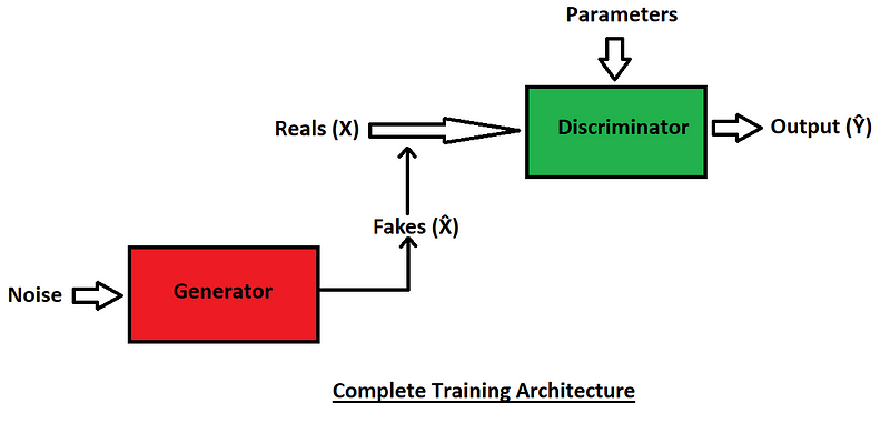
The above block diagram is the representation of the complete training structure. We will focus on the training phases of both the discriminator and the generator independently later on in this section. However, now we will analyze the overall structure and discuss more in detail about the Binary Cross Entropy (BCE) Function, which will be an essential aspect for the rest of the article.
Binary Cross Entropy (BCE) is extremely useful for training GANs. The main purpose of this function is the utility it has for classification tasks for the prediction of real or fake data. Let us look at the overall cost function of the BCE and analyze it further by breaking it down into two parts. The range of the summation ($Σ$) is from $1$ to $m$. The calculation of the left term is considered after the summation symbol and before the addition sign. The right-hand side includes the terms that are everything after the addition symbol.
Cost Function
$$ J(Θ) = -1/m * Σ [y(i) logh(x(i), Θ) + (1 - y(i)) log(1 - h(x(i), Θ))] $$
Alternative View
J(Θ) = -1/m * Σ [y(i) logh(x(i), Θ) + (1-y(i)) log(1-h(x(i),Θ))]
Where,
- $-1/m * Σ$ represents the average loss of the whole batch. The negative sign at the beginning of the equation is to symbolize and always ensure that the cost computed is greater than or equal to zero. Our main objective is to reduce the cost function for producing better results.
- $h$ is the representation of the predictions made.
- $y(i)$ represents the labels of the computations. $y(0)$ could stand for fake images, while $y(1)$ could represent real images.
- $x(i)$ are the features that are calculated.
- $Θ$ is a representation of the parameters that need to be calculated.
LHS: $ y(i) logh(x(i), Θ) $
The left-hand side of the prediction is mostly relevant when the value of the label is one, i.e. when the value of $y(i)$ is real (in our case, $1$). When the value of $y(i)$ is zero, the output of the product of the label and the log function will always be zero. However, when the output label has a value of one, we have two conditions that arise. Let us analyze both situations individually now.
When the components inside the log result in a good prediction, we receive a positive value ranging from $0$ to $1$ (usually a high value like $0.99$). Hence, due to the log function, the final output is $0$. The value after multiplying with the $y(i)$ value also results in $0$. Therefore, we can determine that the left-hand side produces a result of $0$ for a good prediction.
In the second case of a bad prediction, i.e. when the components inside the log result in a bad prediction, we receive a value close to $0$. Hence, due to the log function, the final input is close to negative infinity. The product of $y(i)$ and the log function also results in a high negative value. Therefore, we can determine that the left-hand side produces a result of a high negative number (infinity) for a bad prediction.
RHS: $ (1 — y(i)) log(1 — h(x(i), Θ)) $
Similar to the left-hand side, the right-hand side of the prediction is mostly relevant when the value of the label is zero, i.e. when the value of $y(i)$ is fake (in our case, $0$). When the value of $y(i)$ is one, the output of the product of the label and the log function will always result in a zero. However, when the output label has a value of zero, we have two conditions that arise. Let us analyze both situations individually now.
When the components inside the log result in a good prediction, we receive a positive value ranging from $0$ to $1$ (usually a low value like $0.01$). Hence, due to the log function, the final output is $0$. The value after multiplying with the $(1-y(i))$ value also results in $0$. Therefore, we can determine that the right-hand side produces a result of $0$ for a good prediction.
In the second case of a bad prediction, i.e. when the components inside the log result in a bad prediction, we receive a value close to $0$. Due to the log function, the final input is close to negative infinity. The product of the $(1-y(i))$ value and the log function also results in a high negative value. Therefore, we can determine that the right-hand side produces a high negative number (infinity) for a bad prediction.
To summarize these concepts briefly, when the right predictions are made we receive a value of $0$, while a wrong prediction gives us negative values (usually negative infinity), but the $-1/m$ portion of the equation always turns these negative values into positive ones.
Discriminator Phase
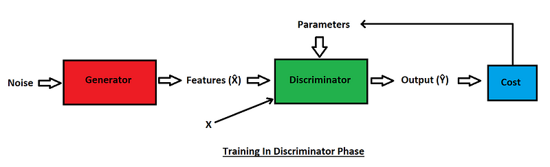
The above block diagram is a representation of training in the Discriminator Phase for Generative Adversarial Networks. Usually, the parameters of the discriminator are initially updated, and then we move onto the generator. We can notice that a random noise sample is passed through the generator block. Since the generator initially has no knowledge of the actual values or output to be produced, we will receive some junk values, which are termed as the features $\hat{X}$ of the generator.
In the next step, both the features of the generator $\hat{X}$ and the actual features $X$ are passed through the discriminator. Initially, the features produced by the generator perform terribly compared to the actual features. The discriminator also performs poorly during the starting stages of the training procedure. Hence, it is essential to update the parameters of the discriminator accordingly.
The output $Ŷ$ results from the discriminator block after the features of the generator are compared against the actual features. The discriminator, as discussed previously, acts similar to a classifier. There is another comparison step, where we once again receive output from the discriminator and compare it with the actual output to calculate the overall cost function. Finally, the parameters of the discriminator are updated accordingly.
Note: It is extremely important to note that during the training phase of the discriminator, only the parameters of the discriminator are updated. The parameters of the generator remain unchanged during this phase.
In other words, both the real and fake images are passed through the discriminator of the GAN to compute an output prediction without telling which images are real or fake. The predicted output is compared with the Binary Cross Entropy (BCE) labels for the predicted category (real or fake – usually, $1$ is used to represent a real image, while $0$ represents a fake one). Finally, after the computation of all these steps, the parameters of the discriminator can be updated accordingly.
Generator Phase
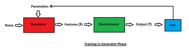
The above diagram is a representation of training in the generator phase. We can notice that in this phase, some noise is provided to the generator, but an equivalent update is made to the parameters of the generators. The parameters are updated accordingly, taken into consideration the feedback that is received from the discriminator. Here, we can also notice that only the features $\hat{X}$ are used for evaluation, while the actual features $X$ are not.
The generator computes only on the real images. No fake images are passed to the generator. The cost function after the calculation is evaluated and the parameters of the generator are updated. In this training phase, only the parameters of the generator are updated accordingly, while the discriminator parameters are neglected.
When the BCE values are equal to real (or $1$), only then are the generated parameters updated. Both the generator and discriminator are trained one at a time, and they are both trained alternately. The generator learns from getting feedback if its classification was right or wrong.
Both the discriminator and generator models should improve together. They should be kept at similar skill levels from the beginning of training. You don’t want a superior discriminator that learns too quickly, because it becomes much better at distinguishing between real and fake, while the generator can never learn fast enough to produce convincing fake images. A similar case occurs when the generator is trained at a faster pace, because then the discriminator fails at its tasks and allows any random image to be generated. Hence, it is essential to ensure that both the generator and discriminators are trained at a consistent pace.
Applications of GANs
- Make yourself or others look younger or older by developing an application based on GANs (e.g. FaceApp)
- Generate realistic pictures of people that have never existed.
- Generate new and unique music.
- Convert low-resolution images and videos to high-resolution.
- Create duplicates of X-rays for medical scans and images, if there is a lack of data.
- Drawings and artistic sketches.
- Animated gifs from normal images.
There are countless more applications for these adversarial networks, and their popularity is currently on the rise, which will lead to many more spectacular applications to come. It is exciting to think about and speculate on the future innovations to be discovered or created with GANs.
Conclusion
In this article, our main objective was to gain an intuitive understanding of how Generative Adversarial Networks (GANs) work. GANs are a remarkable feat of the modern era of deep learning. They provide a unique approach to create and generate data like images and text, and can also perform functions like natural image synthesis, data augmentation, and so much more.
Let's quickly recap the numerous topics we discussed in this article. We had a quick introduction and learned about realistic expectations from GANs, including their usage in industry. We then proceeded to understand the different types of modeling, including discriminative models and generative models. Afterwards, we focused on the two main types of generative models, namely Variational Autoencoders and Generative Adversarial Networks.
We discussed the discriminator and the generator blocks separately and in detail. We identified their respective roles and their purpose in generating new data. They essentially play the role of a thief and a cop, where the generator tries to create perfect (albeit fake) models while the discriminator tries to distinguish and classify between real and fake data. We also looked at examples of their implementations using PyTorch to gain a brief insight into their mechanisms.
We then understood the in-depth training procedure of both the generator and the discriminator independently. We learned how their respective parameters are updated equivalently, such that both the generator and discriminator are balanced. They need to be trained in such a way that they counterbalance each other, and we need to make sure they both improve equally. Finally, we concluded with an understanding of the various applications of GANs in the real world and discovered their impact on our daily lives.
In the next part of the GANs series, we will learn more about the different types of GANs and look in-depth into a special class of GANs called Deep Convolutional Generative Adversarial Networks (DCGANs). Until then, enjoy practicing and learning more!