pix2pix Generative Adversarial Networks

Out of the numerous miracles that Generative Adversarial Networks (GANs) can achieve, such as generating completely new entities from scratch, they also have another fantastic use case for image-to-image translation. In previous blogs, we learned about the implementation of Conditional GANs. These conditional GANs are characterized the ability to perform a task to obtain the required output for the particular input provided to the training network. Before we proceed to one of the variations of these conditional GANs in this article, I would suggest checking CGAN's implementation from this link.

In this article, we will explore one of the variations of GAN that has been gaining tremendous popularity over the recent years due to its ability to translate images from the source to the target domain with high precision: pix2pix GANs. We will start with a brief introduction of the basics required for following this blog before we proceed to understand the pix2pix GAN research paper with an architectural breakdown. Finally, we will develop a satellite image to maps translation project using pix2pix GANs from scratch.

The Paperspace Gradient platform can be utilized to run the following project by creating a Paperspace Gradient Notebook using the following linked repo as the "Workspace URL." This field can be found by toggling the advanced options button on the Notebook creation page.

Introduction:

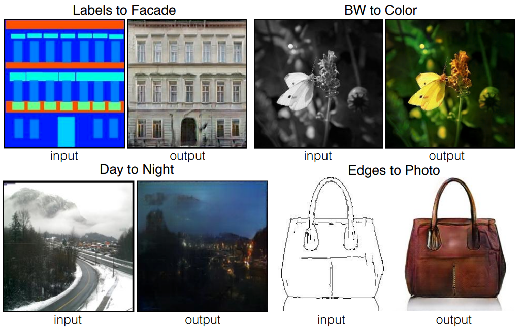
One of the major applications of conditional GANs is the ability of these networks to perform highly precise image-to-image translations. The image-to-image translation is a task in which we take an image from one particular domain and convert it into an image in another domain by transforming it as required for a particular task. There are a variety of image translation projects that one can work on, including the conversion of black and white images to color images, animated sketches to realistic human pictures, and a lot of other similar ideas.

Many methods have been previously utilized to perform image-to-image translations with high precision. However, a naive CNN approach to minimize the Euclidean distance between predicted and ground truth pixels tends to produce blurry results. The main reason for the blurring effect is that the Euclidean distance is minimized by averaging all plausible outputs. The pix2pix conditional GAN fixes most of these underlying issues. The blurry images will be determined as fake samples by the discriminator network, solving a major issue of the previous CNN methods. In the upcoming section, we will gain a more conceptual understanding of these pix2pix conditional GANs.

Understanding pix2pix GANs:

Many methods have been previously used for performing a variety of image translation tasks. However, historically most primitive methods failed, including some from popular deep learning frameworks. Where most methods struggled in generative tasks, Generative Adversarial Networks succeed in most cases. One of the best networks for image translations are the pix2pix GANs. In this section, we will break down the procedural working of these pix2pix GANs, and try to understand the intricate details of the generator and discriminator networks of the pix2pix GAN architecture.

The generator architecture makes use of the U-Net architectural design. We have covered this topic in tremendous detail in one of my previous blogs that you can check out from this link. The U-Net architecture uses an encoder-decoder type structure where we have convolutional layers down-sampled in the first half of the architecture, and the second half involves using upsampling by layers like convolutional transpose to resize to a higher image scaling. The traditional U-Net architecture is slightly older since it was originally developed way back in 2015, and neural networks have advanced massively since then.

Hence, the U-Net architecture used in this generator network of the pix2pix GAN is a slightly modified version of the original U-Net architecture. While the encoder-decoder structure, along with the skip connections, is a crucial aspect of both networks; there are some key noteworthy differences. The image size in the original U-Net architecture changed from the original dimensions to a new lesser height and width. In the pix2pix GAN network, the generator networks preserve the image size and dimensions. We also make use of only one convolutional layer block in the pix2pix generator network before down striding as opposed to the two blocks originally used. Finally, the U-Net network scaled down to a max value of around 32 x 32, whereas the generator network scales down all the way down to 1 x 1.

As for the proposed discriminator architecture, the pix2pix GAN makes use of a patch-wise method that only penalizes structure at the scale of patches. While most complex discriminators in GAN architectures utilize the whole image for establishing a fake or real (0 or 1) value, the patch GAN tries to classify if each N ×N patch in an image is real or fake. The N x N patch size can vary for each specific task, but the ultimate final output is the average of all the responses of the patches considered. The primary advantages of the Patch GAN discriminator occur from the facts that they have fewer training parameters, run faster, and can be applied to arbitrarily large images.

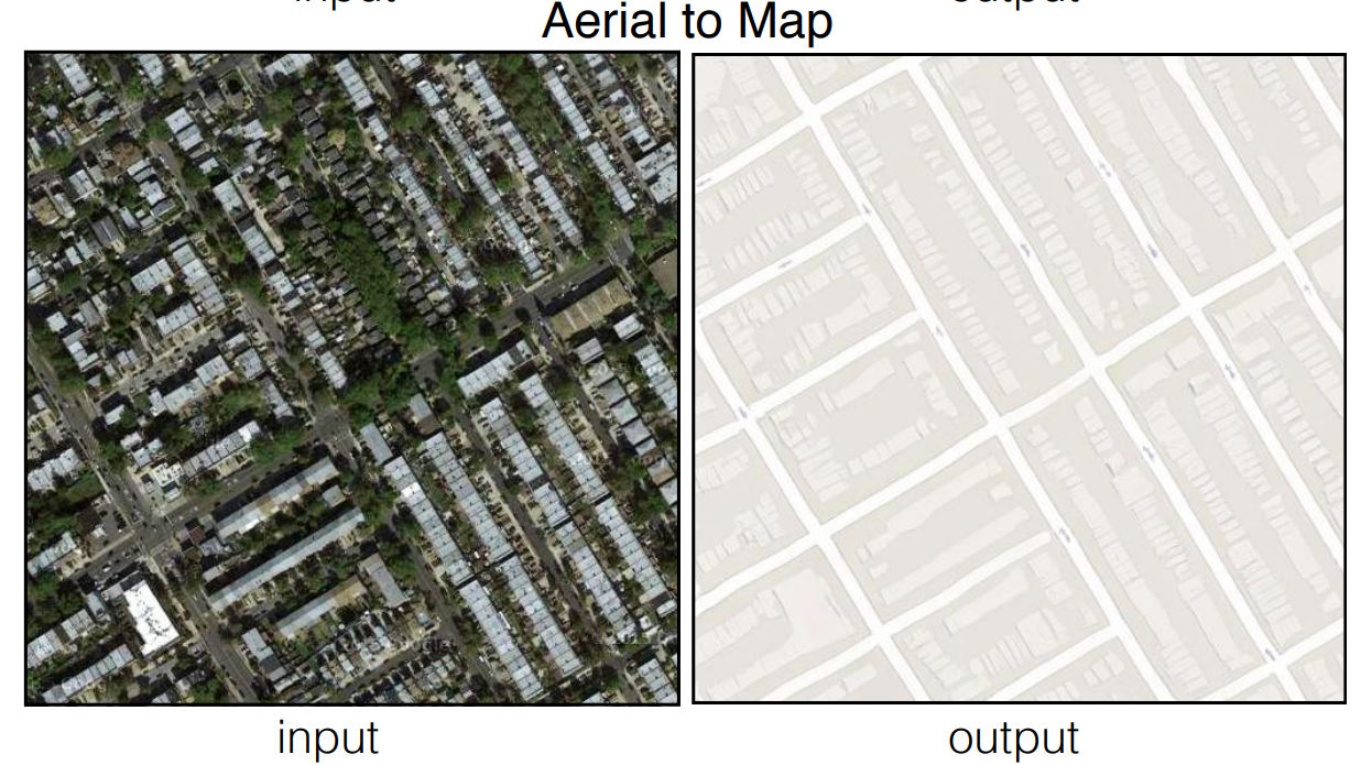
There are numerous experiments that we can perform with the help of pix2pix GANs. Some of these experiments include semantic labels to photo translations on cityscapes, architectural labels to photos on facades dataset, black and white images to colored images, animated sketches to realistic human pictures, and so much more! In this project, we will focus on the satellite map to an aerial photo conversion, trained on data scraped from Google Maps.

Satellite Image to Maps Translation using pix2pix GANs:

In this section of the article, we will focus on developing a pix2pix GAN architecture from scratch for the translation of satellite images to their respective maps. Before getting started with this tutorial, I would highly recommend checking out both my previous blogs on the TensorFlow article as well as the Keras article. These two libraries will be the primary deep learning frameworks that we will utilize for constructing the following project. The project is divided into many smaller sub-sections for gaining an easier understanding of all the steps required to accomplish the desired task. Let us get started by importing all the essential libraries.

Importing the essential libraries

As discussed previously, the two primary deep learning frameworks we will utilize are TensorFlow and Keras. The most useful layers include convolutional layers, Leaky ReLU activation function, batch normalizations, dropout layers, and a few other essential layers. We will also import the NumPy library to work with arrays and generate the real and fake images accordingly. The Matplotlib library is utilized for plotting the required graphs and necessary plots. Check out the below code block for all the required libraries and imports that we will make use of for the construction of this project.

from tensorflow.keras.optimizers import Adam
from tensorflow.keras.initializers import RandomNormal
from tensorflow.keras.models import Model
from tensorflow.keras.layers import Input, Conv2D, Conv2DTranspose, LeakyReLU, Activation
from tensorflow.keras.layers import BatchNormalization, Concatenate, Dropout
from keras.preprocessing.image import img_to_array
from keras.preprocessing.image import load_img
from tensorflow.keras.utils import plot_model
from tensorflow.keras.models import load_model
from os import listdir
from numpy import asarray, load
from numpy import vstack
from numpy import savez_compressed
from matplotlib import pyplot
import numpy as np
from matplotlib import pyplot as plt
from numpy.random import randint
from numpy import zeros
from numpy import ones

Preparing the data:

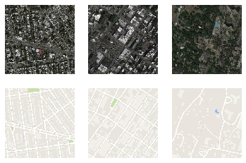
By looking at and analyzing our data, we can notice that we have a whole image containing both the maps and their respective satellite images. In the upcoming code block, we will define the path to our dataset. I would recommend the readers who want to experiment alongside the tutorial download this dataset from Kaggle. The following dataset aims to work as a general-purpose solution for image-to-image translation problems. They have four datasets that we can utilize for developing the Pix2Pix GANs. These datasets include Facades, Cityscapes, Maps, and Edges to shoes.

You can also download any other additional downloads that you want to test the model working procedure on. For this article, we will make use of the maps dataset. In the below code block, I have defined the particular path to my directory that contains the maps data with the train and validation directories. Feel free to set your own path location accordingly. We will also define some of the basic parameters with which some of the coding procedures can be done with a bit more ease. Since the image contains both the satellite image and its respective map, we can split them equally as they are both of the dimension 256 x 256, as shown in the below code block.

# load all images in a directory into memory
def load_images(path, size=(256,512)):
    src_list, tar_list = list(), list()
    for filename in listdir(path):
        # load and resize the image
        pixels = load_img(path + filename, target_size=size)
        # convert to numpy array
        pixels = img_to_array(pixels)
        # split into satellite and map
        sat_img, map_img = pixels[:, :256], pixels[:, 256:]
        src_list.append(sat_img)
        tar_list.append(map_img)
    return [asarray(src_list), asarray(tar_list)]

# dataset path
path = 'maps/train/'
# load dataset
[src_images, tar_images] = load_images(path)
print('Loaded: ', src_images.shape, tar_images.shape)


n_samples = 3
for i in range(n_samples):
    pyplot.subplot(2, n_samples, 1 + i)
    pyplot.axis('off')
    pyplot.imshow(src_images[i].astype('uint8'))
    
# plot target image
for i in range(n_samples):
    pyplot.subplot(2, n_samples, 1 + n_samples + i)
    pyplot.axis('off')
    pyplot.imshow(tar_images[i].astype('uint8'))
pyplot.show()

Loaded:  (1096, 256, 256, 3) (1096, 256, 256, 3)

U-Net Generator Network:

For constructing the generator network of the pix2pix GAN architecture, we will divide the structure into a few parts. We will start with the encoder block, where we will define the convolutional layers with a striding of two, followed by the Leaky ReLU activation function. Most of the convolutional layers will also be followed by the batch normalization layers, as shown in the below code block. Once we return the encoder block of the generator network, we can construct the first half of the network as follows - C64-C128-C256-C512-C512-C512-C512-C512.

# Encoder Block
def define_encoder_block(layer_in, n_filters, batchnorm=True):
    init = RandomNormal(stddev=0.02)
    g = Conv2D(n_filters, (4,4), strides=(2,2), padding='same', kernel_initializer=init)(layer_in)
    if batchnorm:
        g = BatchNormalization()(g, training=True)
    g = LeakyReLU(alpha=0.2)(g)
    return g

The next part of the generator network we will define is the decoder block. In this function, we will upsample all the previously downsampled images as well as add (concatenate) the necessary skip connections that must be made from the encoder to the decoder network, similar to the U-Net architecture. For the upsampling of the model, we can make use of the convolutional transpose layers with batch normalization layers and optional dropout layers. The decoder block of the generator network contains the architecture as follows - CD512-CD512-CD512-C512-C256-C128-C64. Below is the code block for the following structure.

# Decoder Block
def decoder_block(layer_in, skip_in, n_filters, dropout=True):
    init = RandomNormal(stddev=0.02)
    g = Conv2DTranspose(n_filters, (4,4), strides=(2,2), padding='same', kernel_initializer=init)(layer_in)
    g = BatchNormalization()(g, training=True)
    if dropout:
        g = Dropout(0.5)(g, training=True)
    # merge with skip connection
    g = Concatenate()([g, skip_in])
    g = Activation('relu')(g)
    return g

Now that we have constructed our previous two primary functions, namely the encoder and decoder block, we can proceed to call them multiple times to align the network as per the necessary requirement. We will follow the encoder and decoder network architecture as we previously discussed in this section and construct these blocks accordingly. Most of the structure is built in accordance with the following research paper. The final output activation function tanh generates images in the range -1 to 1. Feel free to try out any other smaller modifications that could potentially result in yielding better results by modifying some of the parameters. The code block for the generator network is provided below.

# Define the overall generator architecture
def define_generator(image_shape=(256,256,3)):
    # weight initialization
    init = RandomNormal(stddev=0.02)
    
    # image input
    in_image = Input(shape=image_shape)
    
    # encoder model: C64-C128-C256-C512-C512-C512-C512-C512
    e1 = define_encoder_block(in_image, 64, batchnorm=False)
    e2 = define_encoder_block(e1, 128)
    e3 = define_encoder_block(e2, 256)
    e4 = define_encoder_block(e3, 512)
    e5 = define_encoder_block(e4, 512)
    e6 = define_encoder_block(e5, 512)
    e7 = define_encoder_block(e6, 512)
    
    # bottleneck, no batch norm and relu
    b = Conv2D(512, (4,4), strides=(2,2), padding='same', kernel_initializer=init)(e7)
    b = Activation('relu')(b)
    
    # decoder model: CD512-CD512-CD512-C512-C256-C128-C64
    d1 = decoder_block(b, e7, 512)
    d2 = decoder_block(d1, e6, 512)
    d3 = decoder_block(d2, e5, 512)
    d4 = decoder_block(d3, e4, 512, dropout=False)
    d5 = decoder_block(d4, e3, 256, dropout=False)
    d6 = decoder_block(d5, e2, 128, dropout=False)
    d7 = decoder_block(d6, e1, 64, dropout=False)
    
    # output
    g = Conv2DTranspose(image_shape[2], (4,4), strides=(2,2), padding='same', kernel_initializer=init)(d7) #Modified 
    out_image = Activation('tanh')(g)  #Generates images in the range -1 to 1. So change inputs also to -1 to 1
    
    # define model
    model = Model(in_image, out_image)
    return model

Patch GAN discriminator Network:

Once the generator network is constructed, we can proceed to work on the discriminator architecture. We will initialize our weights and merge the input source image and the target image before proceeding to build the discriminator structure. The discriminator structure will follow the pattern build of C64-C128-C256-C512. After the last layer, a convolution is applied for mapping to a 1-dimensional output, followed by the sigmoid function. The discriminator network used in the below code block allows the size to go down as low as 16 x 16. Finally, we can compile the model that is trained with a batch size of one image and the Adam optimizer with a small learning rate and 0.5 beta value. The loss for the discriminator is weighted by 50% for each model update. Check the below code snippet for the full patch GAN discriminator network.

def define_discriminator(image_shape):
    
    # weight initialization
    init = RandomNormal(stddev=0.02)
    
    # source image input
    in_src_image = Input(shape=image_shape)  
    
    # target image input
    in_target_image = Input(shape=image_shape)  
    
    # concatenate images, channel-wise
    merged = Concatenate()([in_src_image, in_target_image])
    
    # C64: 4x4 kernel Stride 2x2
    d = Conv2D(64, (4,4), strides=(2,2), padding='same', kernel_initializer=init)(merged)
    d = LeakyReLU(alpha=0.2)(d)
    
    # C128: 4x4 kernel Stride 2x2
    d = Conv2D(128, (4,4), strides=(2,2), padding='same', kernel_initializer=init)(d)
    d = BatchNormalization()(d)
    d = LeakyReLU(alpha=0.2)(d)
    
    # C256: 4x4 kernel Stride 2x2
    d = Conv2D(256, (4,4), strides=(2,2), padding='same', kernel_initializer=init)(d)
    d = BatchNormalization()(d)
    d = LeakyReLU(alpha=0.2)(d)
    
    # C512: 4x4 kernel Stride 2x2 
    d = Conv2D(512, (4,4), strides=(2,2), padding='same', kernel_initializer=init)(d)
    d = BatchNormalization()(d)
    d = LeakyReLU(alpha=0.2)(d)
    
    # second last output layer : 4x4 kernel but Stride 1x1 (Optional)
    d = Conv2D(512, (4,4), padding='same', kernel_initializer=init)(d)
    d = BatchNormalization()(d)
    d = LeakyReLU(alpha=0.2)(d)
    
    # patch output
    d = Conv2D(1, (4,4), padding='same', kernel_initializer=init)(d)
    patch_out = Activation('sigmoid')(d)
    
    # define model
    model = Model([in_src_image, in_target_image], patch_out)
    opt = Adam(lr=0.0002, beta_1=0.5)
    
    # compile model
    model.compile(loss='binary_crossentropy', optimizer=opt, loss_weights=[0.5])
    return model

Define the complete GAN architecture:

Now that we have defined both the generator and the discriminator network, we can proceed to train the entire GAN architecture as desired. The weights in the discriminator are not trainable, but the standalone discriminator is trainable. Hence, we will set these parameters accordingly. We will then pass the source image as the input to the model, while the output of the model will contain both the generated results as well the discriminator output. The total loss is computed as the weighted sum of adversarial loss (BCE) and L1 loss (MAE), with weights in the ratio of 1:100. We can compile the model with these parameters and the Adam optimizer to return the final model.

# define the combined GAN architecture
def define_gan(g_model, d_model, image_shape):
    for layer in d_model.layers:
        if not isinstance(layer, BatchNormalization):
            layer.trainable = False
            
    in_src = Input(shape=image_shape)
    gen_out = g_model(in_src)
    dis_out = d_model([in_src, gen_out])
    model = Model(in_src, [dis_out, gen_out])
    # compile model
    opt = Adam(lr=0.0002, beta_1=0.5)
    
    model.compile(loss=['binary_crossentropy', 'mae'], 
               optimizer=opt, loss_weights=[1,100])
    
    return model

Defining all the essential parameters:

In the next step, we will define all the essential functions and parameters that we will require for training the pix2pix GAN model. Firstly, let us define the functions to generate the real and fake samples. The code snippet for performing the following action is provided below.

def generate_real_samples(dataset, n_samples, patch_shape):
    trainA, trainB = dataset
    ix = randint(0, trainA.shape[0], n_samples)
    X1, X2 = trainA[ix], trainB[ix]
    y = ones((n_samples, patch_shape, patch_shape, 1))
    return [X1, X2], y

def generate_fake_samples(g_model, samples, patch_shape):
    X = g_model.predict(samples)
    y = zeros((len(X), patch_shape, patch_shape, 1))
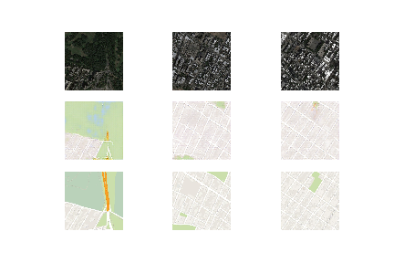
    return X, y

In the next code block, we will create a function for summarizing the performance of our model. The generated images will be compared with their original counterparts to receive the desired response. We can plot three graphs for the source image, the generated image, and the target output image. We can save the plot and the generator model to utilize later for further computations as desired.

#save the generator model and check how good the generated image looks. 
def summarize_performance(step, g_model, dataset, n_samples=3):
    [X_realA, X_realB], _ = generate_real_samples(dataset, n_samples, 1)
    X_fakeB, _ = generate_fake_samples(g_model, X_realA, 1)
    
    # scale all pixels from [-1,1] to [0,1]
    X_realA = (X_realA + 1) / 2.0
    X_realB = (X_realB + 1) / 2.0
    X_fakeB = (X_fakeB + 1) / 2.0
    
    # plot real source images
    for i in range(n_samples):
        plt.subplot(3, n_samples, 1 + i)
        plt.axis('off')
        plt.imshow(X_realA[i])
        
    # plot generated target image
    for i in range(n_samples):
        plt.subplot(3, n_samples, 1 + n_samples + i)
        plt.axis('off')
        plt.imshow(X_fakeB[i])
        
    # plot real target image
    for i in range(n_samples):
        plt.subplot(3, n_samples, 1 + n_samples*2 + i)
        plt.axis('off')
        plt.imshow(X_realB[i])
        
    # save plot to file
    filename1 = 'plot_%06d.png' % (step+1)
    plt.savefig(filename1)
    plt.close()
    
    # save the generator model
    filename2 = 'model_%06d.h5' % (step+1)
    g_model.save(filename2)
    print('>Saved: %s and %s' % (filename1, filename2))

Finally, let us define the train function through which we can train the model and call all the appropriate functions for generating samples, summarizing model performance, and the training on batch functions as required. Once we have created the training function for the pix2pix model, we can proceed to train the model and generate the results for the satellite image to maps image translation task. Below is the code block for the train function.

# train function for the pix2pix model
def train(d_model, g_model, gan_model, dataset, n_epochs=100, n_batch=1):
    n_patch = d_model.output_shape[1]
    trainA, trainB = dataset
    bat_per_epo = int(len(trainA) / n_batch)
    n_steps = bat_per_epo * n_epochs
    
    for i in range(n_steps):
        [X_realA, X_realB], y_real = generate_real_samples(dataset, n_batch, n_patch)
        X_fakeB, y_fake = generate_fake_samples(g_model, X_realA, n_patch)
        
        d_loss1 = d_model.train_on_batch([X_realA, X_realB], y_real)
        d_loss2 = d_model.train_on_batch([X_realA, X_fakeB], y_fake)
        g_loss, _, _ = gan_model.train_on_batch(X_realA, [y_real, X_realB])
        
        # summarize model performance
        print('>%d, d1[%.3f] d2[%.3f] g[%.3f]' % (i+1, d_loss1, d_loss2, g_loss))
        if (i+1) % (bat_per_epo * 10) == 0:
            summarize_performance(i, g_model, dataset)

Training the pix2pix model:

Once we have constructed the entire generator and discriminator network and combined them into the GAN architecture as well as finished declaring all the essential parameters and values, we can proceed to finally train the pix2pix model and observe its performance. We will pass the image shape of the source and construct the GAN architecture with respect to the generator and discriminator network.

We will define the input source images and target images and then normalize these images accordingly to scale them in the desired range of -1 to 1 as the output tanh activation function will perform. We can finally begin the training of the model and evaluate the performance after ten epochs. The parameters are reported for each batch (total of 1096) for each epoch. For ten epochs, we should notice a total of 10960. Below is the code snippet for training the model.

image_shape = src_images.shape[1:]
d_model = define_discriminator(image_shape)
g_model = define_generator(image_shape)
gan_model = define_gan(g_model, d_model, image_shape)

data = [src_images, tar_images]

def preprocess_data(data):
    X1, X2 = data[0], data[1]
    # scale from [0,255] to [-1,1]
    X1 = (X1 - 127.5) / 127.5
    X2 = (X2 - 127.5) / 127.5
    return [X1, X2]

dataset = preprocess_data(data)

from datetime import datetime 
start1 = datetime.now() 

train(d_model, g_model, gan_model, dataset, n_epochs=10, n_batch=1) 

stop1 = datetime.now()
#Execution time of the model 
execution_time = stop1-start1
print("Execution time is: ", execution_time)

>10955, d1[0.517] d2[0.210] g[8.743]
>10956, d1[0.252] d2[0.693] g[5.987]
>10957, d1[0.243] d2[0.131] g[12.658]
>10958, d1[0.339] d2[0.196] g[6.857]
>10959, d1[0.010] d2[0.125] g[4.013]
>10960, d1[0.085] d2[0.100] g[10.957]
>Saved: plot_010960.png and model_010960.h5
Execution time is:  0:39:10.933599

The execution of the program for the training of the model took around 40 minutes on my system. The time of training can vary depending on your GPU and the features of your device. The Gradient platform on Paperspace is a great viable option for such training mechanisms. After the training is complete, we have a model and a plot available to use. The model can be loaded, and the necessary predictions can be made on it accordingly. Below is the code block for loading the model as well as making the essential predictions along with their respective plots.

# Plotting the Final Results
model = load_model('model_010960.h5')

# plot source, generated and target images
def plot_images(src_img, gen_img, tar_img):
    images = vstack((src_img, gen_img, tar_img))
    # scale from [-1,1] to [0,1]
    images = (images + 1) / 2.0
    titles = ['Source', 'Generated', 'Expected']
    
    # plot images row by row
    for i in range(len(images)):
        pyplot.subplot(1, 3, 1 + i)
        pyplot.axis('off')
        pyplot.imshow(images[i])
        pyplot.title(titles[i])
    pyplot.show()

[X1, X2] = dataset
# select random example
ix = randint(0, len(X1), 1)
src_image, tar_image = X1[ix], X2[ix]
# generate image from source
gen_image = model.predict(src_image)
# plot all three images
plot_images(src_image, gen_image, tar_image)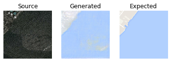

I would highly recommend checking out the following website from which a majority of the code has been considered. As the next step, it is highly recommended that the viewers try out numerous combinations that could maybe help in producing even better results. The viewers can also choose to implement the training for a higher number of epochs to try and achieve a more desirable result. Apart from this project, pix2pix GANs find a high utility in a variety of projects. I would suggest trying out numerous projects to get a better hang on the capabilities of these generative networks.

Conclusion:

Image-To-Image translation from one image to another is quite a complex task as simple convolutional networks fail to accomplish this task in the most desirable manner due to their lack of feature extraction ability. GANs, on the other hand, do an exceptional job at generating some of the best images with high precision and accuracy. They also help in avoiding some of the lackluster effects of simple convolutional networks, such as output sharp, realistic images, etc. Hence, the introduced pix2pix GAN architecture is one of the best versions of GAN to solve such problems. The pix2pix GAN software is even utilized by artists and multiple users via the internet to achieve high-quality results.

In this article, we focused on one of the most significant types of conditional type GANs in pix2pix GANs for image translation. We learned more about the topic of image translation and understood most of the basic concepts related to pix2pix GANs and their mechanism of function. Once we covered the essential aspects of the pix2pix GAN, including the generator and discriminator architecture, we proceeded to construct the satellite image translation to maps project. It is highly recommended that the viewers try out other similar projects as well as try out some of the numerous possibilities of the different types of variations possible with the generator and discriminator network of the pix2pix GAN architecture.

In future articles, we will focus on building more projects with pix2pix GANs as there are numerous possibilities with these conditional networks. We will also explore other types of GANs like Cycle GANs as well as other tutorials and projects on BERT transformers and Constructing Neural Networks From Scratch (Part-2). Until then, enjoy coding and building new projects!