In Part 1 of our series on how to write efficient code using NumPy, we covered the important topics of vectorization and broadcasting. In this part we will put these concepts into practice by implementing an efficient version of the K-Means clustering algorithm using NumPy. We will benchmark it against a naive version implemented entirely using looping in Python. In the end we'll see that the NumPy version is about 70 times faster than the simple loop version.
To be exact, in this post we will cover:
- Understanding K-Means Clustering
- Implementing K-Means using loops
- Using cProfile to find bottlenecks in the code
- Optimizing K-Means using NumPy
Let's get started!
Bring this project to life
Understanding K-Means Clustering
In this post we will be optimizing an implementation of the k-means clustering algorithm. It is therefore imperative that we at least have a basic understanding of how the algorithm works. Of course, a detailed discussion would also be beyond the scope of this post; if you want to dig deeper into k-means you can find several recommended links below.
What Does the K-Means Clustering Algorithm Do?
In a nutshell, k-means is an unsupervised learning algorithm which separates data into groups based on similarity. As it's an unsupervised algorithm, this means we have no labels for the data.
The most important hyperparameter for the k-means algorithm is the number of clusters, or k. Once we have decided upon our value for k, the algorithm works as follows.
- Initialize k points (corresponding to k clusters) randomly from the data. We call these points centroids.
- For each data point, measure the L2 distance from the centroid. Assign each data point to the centroid for which it has the shortest distance. In other words, assign the closest centroid to each data point.
- Now each data point assigned to a centroid forms an individual cluster. For k centroids, we will have k clusters. Update the value of the centroid of each cluster by the mean of all the data points present in that particular cluster.
- Repeat steps 1-3 until the maximum change in centroids for each iteration falls below a threshold value, or the clustering error converges.
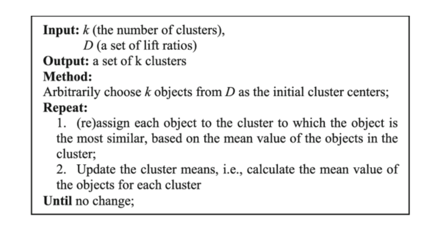
Here's the pseudo-code for the algorithm.
I'm going to leave K-Means at that. This is enough to help us code the algorithm. However, there is much more to it, such as how to choose a good value of k, how to evaluate the performance, which distance metrics can be used, preprocessing steps, and theory. In case you wish to dig deeper, here are a few links for you to study it further.
 Imad Dabbura
Now, let's proceed with the implementation of the algorithm.
Implementing K-Means Using Loops
In this section we will be implementing the K-Means algorithm using Python and loops. We will not be using NumPy for this. This code will be used as a benchmark for our optimized version.
Generating the Data
To perform clustering, we first need our data. While we can choose from multiple datasets online, let's keep things rather simple and intuitive. We are going to synthesize a dataset by sampling from multiple Gaussian distributions, so that visualizing clusters is easy for us.
In case you don't know what a Gaussian distribution is, check it out!


We will create data from four Gaussian's with different means and distributions.
import numpy as np
# Size of dataset to be generated. The final size is 4 * data_size
data_size = 1000
num_iters = 50
num_clusters = 4

# sample from Gaussians
data1 = np.random.normal((5,5,5), (4, 4, 4), (data_size,3))
data2 = np.random.normal((4,20,20), (3,3,3), (data_size, 3))
data3 = np.random.normal((25, 20, 5), (5, 5, 5), (data_size,3))
data4 = np.random.normal((30, 30, 30), (5, 5, 5), (data_size,3))

# Combine the data to create the final dataset
data = np.concatenate((data1,data2, data3, data4), axis = 0)

# Shuffle the data
np.random.shuffle(data)
In order to aid our visualization, let's plot this data in a 3-D space.
import matplotlib.pyplot as plt
from mpl_toolkits.mplot3d import Axes3D

fig = plt.figure()
ax = fig.add_subplot(111, projection='3d')
ax.set_xlabel('x')
ax.set_ylabel('y')
ax.set_zlabel('z')

ax.scatter(data[:,0], data[:,1], data[:,2], s= 0.5)
plt.show()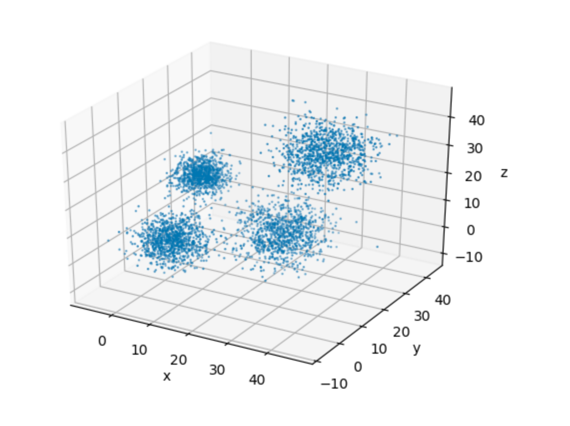
It's very easy to see the four clusters of data in the plot above. This, for one, makes it easy for us to pick up a suitable value of k for our implementation. This goes in spirit of keeping the algorithmic details as simple as possible, so that we can focus on the implementation.
Helper Functions
We begin by initialising our centroids, as well as a list to keep track of which centroid each data point is assigned to.
# Set random seed for reproducibility
random.seed(0)

# Initialize the list to store centroids
centroids = []

# Sample initial centroids
random_indices = random.sample(range(data.shape[0]), 4)
for i in random_indices:
    centroids.append(data[i])

# Create a list to store which centroid is assigned to each dataset
assigned_centroids = [0] * len(data)
Before we implement our loop, we will first implement a few helper functions.
compute_l2_distance takes two points (say [0, 1, 0] and [4, 2, 3]) and computes the L2 distance between them, according to the following formula.
$$ L2(X_1, X_2) = \sum_{i}^{dimensions(X_1)} (X_1[i] - X_2[i])^2 $$
def compute_l2_distance(x, centroid):
    # Initialize the distance to 0
    dist = 0

    # Loop over the dimensions. Take squared difference and add to 'dist'
    for i in range(len(x)):
        dist += (centroid[i] - x[i])**2

    return dist
The other helper function we implement is called get_closest_centroid, the name being pretty self-explanatory. The function takes an input x and a list, centroids, and returns the index of the list centroids corresponding to the centroid closest to x.
def get_closest_centroid(x, centroids):
    # Initialize the list to keep distances from each centroid
    centroid_distances = []

    # Loop over each centroid and compute the distance from data point.
    for centroid in centroids:
        dist = compute_l2_distance(x, centroid)
        centroid_distances.append(dist)

    # Get the index of the centroid with the smallest distance to the data point
    closest_centroid_index =  min(range(len(centroid_distances)), key=lambda x: centroid_distances[x])

    return closest_centroid_index
Then we implement the function compute_sse, which computes the SSE or Sum of Squared Errors. This metric is used to guide how many iterations we have to do. Once this value converges, we can stop training.
def compute_sse(data, centroids, assigned_centroids):
    # Initialise SSE
    sse = 0

    # Compute the squared distance for each data point and add.
    for i,x in enumerate(data):
    	# Get the associated centroid for data point
        centroid = centroids[assigned_centroids[i]]

        # Compute the distance to the centroid
        dist = compute_l2_distance(x, centroid)

        # Add to the total distance
        sse += dist

    sse /= len(data)
    return sse
Main Loop
Now, let's write the main loop. Refer to the pseudo-code mentioned above for reference. Instead of looping until convergence, we merely loop for 50 iterations.
# Number of dimensions in centroid
num_centroid_dims = data.shape[1]

# List to store SSE for each iteration
sse_list = []

tic = time.time()

# Loop over iterations
for n in range(num_iters):

    # Loop over each data point
    for i in range(len(data)):
        x = data[i]

        # Get the closest centroid
        closest_centroid = get_closest_centroid(x, centroids)

        # Assign the centroid to the data point.
        assigned_centroids[i] = closest_centroid

    # Loop over centroids and compute the new ones.
    for c in range(len(centroids)):
        # Get all the data points belonging to a particular cluster
        cluster_data = [data[i] for i in range(len(data)) if assigned_centroids[i] == c]

        # Initialize the list to hold the new centroid
        new_centroid = [0] * len(centroids[0])

        # Compute the average of cluster members to compute new centroid
        # Loop over dimensions of data
        for dim in range(num_centroid_dims):
            dim_sum = [x[dim] for x in cluster_data]
            dim_sum = sum(dim_sum) / len(dim_sum)
            new_centroid[dim] = dim_sum

        # assign the new centroid
        centroids[c] = new_centroid

    # Compute the SSE for the iteration
    sse = compute_sse(data, centroids, assigned_centroids)
    sse_list.append(sse)
The entire code can be viewed below.
Once we let the code run, let's check how we have performed according to the SSE through the iterations.
plt.figure()
plt.xlabel("Iterations")
plt.ylabel("SSE")
plt.plot(range(len(sses)), sses)
plt.show()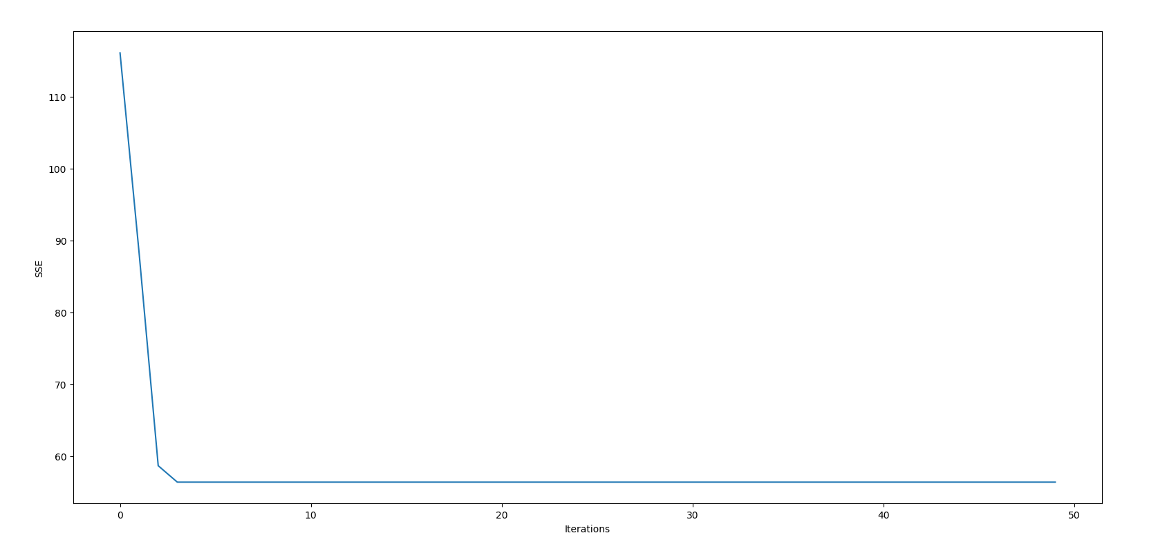
If we visualize the clusters, this is what we get.
fig = plt.figure()
ax = fig.add_subplot(111, projection='3d')


for c in range(len(centroids)):
        cluster_members = [data[i] for i in range(len(data)) if assigned_centroids[i] == c]
        cluster_members = np.array(cluster_members)

        ax.scatter(cluster_members[:,0], cluster_members[:,1], cluster_members[:,2], s= 0.5)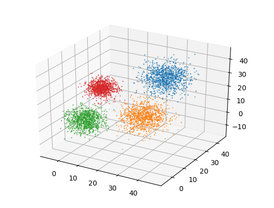
We see that k-means is able to discover all the clusters on its own. We will be using this code as our benchmark.
Timing the Code
Let us now time our code. We can use the timeit module as we did in the last post. You could also use the time module, although in our last post I advocated against it because measuring the running time for only a single run can lead to unstable estimates due to processes running in the background, especially when it comes to short snippets (often, one-liners).
However, it's important to note that the code for K-Means doesn't correspond to a short snippet. In fact, the body of code being considered here has a lot of short snippets being repeated multiple times in loops. This is exactly what we were doing with timeit; running short snippets time and time again. Therefore, even the time module works fine for our example.
In fact, this is what we are going to use here, as shown below.
import time

tic = time.time()

# code to be timed goes here

toc = time.time()

print("Time Elapsed Per Loop {:.3f}".format((tic - toc)/ 50))
When used for our code, the time taken for the loop version is about 0.053 seconds per loop. (Estimates may vary to the tune of 0.001 seconds).
Identifying Bottlenecks
We use a couple of methods to identify bottlenecks: inspection of the loop structure, and the use of cProfile to measure the running time of various functions in our code.
Analyzing the Loop Structure
First, I want to focus on the body of the loop. Here's a rough outline of how loops are structured in the code.
Loop that goes over iteration (n iters)
    .
    .
    # Get centroids for each data point
    Loop that goes over the data (i iters)
    	.
        .
        # Computing distance to centroids
        Loop over centroids (k iters)
            .
            .
            Loop over dimensions of data (d iters)
    .
    .
    # Getting members of the cluster
    Loop over centroids (c iters)
    	.
        .
        # Computing new centroids
        Loop over dimensions of data (d iters)
    .
    .
    # Compute SSE
    Loop over data (i iters)
    	.
        .
        # Compute L2 distance
        Loop over dimensions of data (d iters)
We use n to iterate over the number of iterations, i to iterate over the dataset, c to iterate over the number of clusters, and d to iterate over the dimensions of the data.
Here, the loops that will benefit the most from optimization are those that go over the data (n corresponds to the size of our dataset, which could be very large) and dimensions (d, in case we have very high-dimensional data, like images). In comparison, the loops that go over the number of clusters, c, and the number of iterations, n, may require only a small amount of iterations and may not benefit as much from optimization. Nonetheless, we will try to optimize those as well.
Also notice that the loop that is responsible for calculating the centroids for each data point is a triply nested loop, with individual loops going over the dataset size, number of clusters, and dimensions of the data, respectively. As we've discovered in the previous post, nested loops can be one of the biggest bottlenecks.
Using cProfile to Identify the Bottlenecks
While we could draw an outline detailing loop structure for our code, as it was still somewhat small, doing the same for large bodies of code can be pretty tedious.
Therefore, I am now going to introduce a tool called cProfile that helps you profile your code and get running times for various elements in your code. In order to use cProfile, put your code inside a python script and run the following command from the terminal.
python -m cProfile -o loops.log kmeans_loop.pyHere, -o flag denotes the name of the log file that will be created. In our case, this file is named as loops.log. In order to read this file, we will be needing another utility called cProfileV which can be installed with pip.
pip install cprofilevOnce you have installed it, we can use it to view our log file.
cprofilev -f loops.logThis will result in a message that reads something like:
[cProfileV]: cProfile output available at http://127.0.0.1:4000
Go to the address in the browser. You will see something like this.
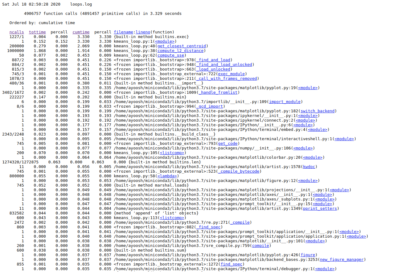
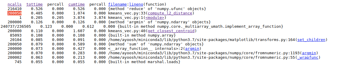
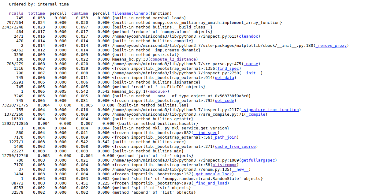
Here, you see column heading on the top regarding each function call in your code.
ncalls: Number of function calls made.tottime: Total time taken by a function call including time taken by other function it calls.percall: Time taken per call.cumtime: Total time taken by the function alone not including time taken by function it calls.filename/lineno: File name and Line number of the function call.
Here, we are most interesting in the time a function call takes by itself, i.e. tottime. We click on the column label to sort the entries by tottime

Once, we have done that we see exactly which functions are taking the most time.
Here, we see that that the function compute_l2_distance and get_closest_centroid take the maximum individual times. Notice that both of these function include loops which can be vectorized. The compute_l2_distance is called 1 million times, while get_closest_centroid is called 200,000 times.
We also see that the <listcomp> (list comprehension function) and the lambda functions also feature in the top time-taking functions. These functions are used in the lines 104, 57, 112 which includes loops for computing data points belonging to a particular cluster, computing the closest centroid and computing the new centroids respectively. We shall also attempt to vectorize these loops.
Optimizing K-Means Algorithm Using NumPy
In this section, we are going to take the implementation and optimize it using vectorization and Broadcasting.
Vectorizing Helper Functions
We first begin by vectorizing the function compute_l2_distance. We modify it to accept inputs x , an array of shape (1, d) (d = 3 in our example) and centroids to be of shape (k, d) (k = 4 in our example).
Since x is of shape (1,3) and centroids of shape (4,3), the array x will be broadcasted over the first dimension and we would have the resulting array of shape (4,3) with each row representing the distance of array x with each centroid. This vectorizes the loop over the number of centroids.
We then sum the resulting (4,3) array along it's first dimensions ( sum(axis = 0)) so that we have an array of size (3,) which contains the distance of x from 3 centroids.
def compute_l2_distance_old(x, centroid):
    # Initialise the distance to 0
    dist = 0

    # Loop over the dimensions. Take sqaured difference and add to `dist`
    for i in range(len(x)):
        dist += (centroid[i] - x[i])**2

    return dist

def compute_l2_distance(x, centroid):

    # Compute the difference, following by raising to power 2 and summing
    dist = ((x - centroid) ** 2).sum(axis = 1)
Now, we turn our attention to the get_closest_centroid function. Again, the inputs to this function would be x , an array of shape (1, d) (d = 3 in our example) and centroids to be of shape (k, d) (k = 4 in our example).
We replace the line closest_centroid_index = min(range(len(centroid_distances)), key=lambda x: centroid_distances[x]) with np.argmin(dist, axis = 0). Note that this lambda call featured in one of top time-taking functions.
def get_closest_centroid_old(x, centroids):
    # Initialise the list to keep distances from each centroid
    centroid_distances = []

    # Loop over each centroid and compute the distance from data point.
    for centroid in centroids:
        dist = compute_l2_distance(x, centroid)
        centroid_distances.append(dist)

    # Get the index of the centroid with the smallest distance to the data point
    closest_centroid_index =  min(range(len(centroid_distances)), key=lambda x: centroid_distances[x])

    return closest_centroid_index

def get_closest_centroid(x, centroids):

    # Loop over each centroid and compute the distance from data point.
    dist = compute_l2_distance(x, centroids)

    # Get the index of the centroid with the smallest distance to the data point
    closest_centroid_index =  np.argmin(dist, axis = 0)

    return closest_centroid_index
Consequently, we can also vectorize the loop in compute_sse function by invoking the compute_l2_distance on the entire data and centroids array.
def compute_sse(data, centroids, assigned_centroids):
    # Initialise SSE
    sse = 0

    # Compute the squared distance for each data point and add.
    for i,x in enumerate(data):
    	# Get the associated centroid for data point
        centroid = centroids[assigned_centroids[i]]

        # Compute the Distance to the centroid
        dist = compute_l2_distance(x, centroid)

        # Add to the total distance
        sse += dist

    sse /= len(data)
    return sse


def compute_sse(data, centroids, assigned_centroids):
    # Initialise SSE
    sse = 0

    # Compute SSE
    sse = compute_l2_distance(data, centroids[assigned_centroids]).sum() / len(data)

    return sse
Note that the data array is of shape (N, 3) (N = 4000). The array centroids[assigned_centroids] helps us get a list of assigned centroids which earlier had to be computed using a loop with the line centroid = centroids[assigned_centroids[i]].
Adjusting the Loop
In order to make the loop work with our modifications, we have to make some modifications to our code.
First, centroids is now a array of shape (4,3) (as compared to a list seen earlier). So we have to change its initialization from:
# Initialise the list to store centroids
centroids = []

# Sample initial centroids
random_indices = random.sample(range(data.shape[0]), 4)
for i in random_indices:
    centroids.append(data[i])
To:
centroids = data[random.sample(range(data.shape[0]), 4)]We also have to ensure our data x is now in form of [1,k] not [k,]. To do this , we add the line x = x[None, :] after reading our data x = data[i].
We also modify the loop that computes the mean of the assigned centroids ( to compute new centroids) to much easier code from
for c in range(len(centroids)):
    # Get all the data points belonging to a particular cluster
    cluster_data = [data[i] for i in range(len(data)) if assigned_centroids[i] == c]

    # Initialise the list to hold the new centroid
    new_centroid = [0] * len(centroids[0])

    # Compute the average of cluster members to compute new centroid
    # Loop over dimensions of data
    for dim in range(num_centroid_dims):
        dim_sum = [x[dim] for x in cluster_data]
        dim_sum = sum(dim_sum) / len(dim_sum)
        new_centroid[dim] = dim_sum

    # assign the new centroid
    centroids[c] = new_centroid
To:
# Loop over centroids and compute the new ones.
for c in range(len(centroids)):
    # Get all the data points belonging to a particular cluster
    cluster_data = data[assigned_centroids == c]

    # Compute the average of cluster members to compute new centroid
    new_centroid = cluster_data.mean(axis = 0)

    # assign the new centroid
    centroids[c] = new_centroid
Once this is done, our new code for K-Means looks like:
Timing the new code
When we time the vectorized code, we get a time of about 0.031 seconds (+/- 0.001 sec). Well, it's a speed up, but isn't it disappointing? To be honest, A speed up of just 1.7x seems to be a big let off given what we saw in Part 1 of one. It seems that maybe vectorization doesn't work that well at all?
Let's use the profiler to see what the time taking functions are.
Again, the functions that take most time (excluding internal functions) are compute_l2_distance and get_closest_centroid. While we vectorized them, a more problematic aspect is them being called a huge number of times. While the compute_l2_distance is now called 200,000 times (instead of 1M due to vectorizing loop over centroids), the number of calls made to get_closest_centroid remains the same.
These large number of calls are because we are still using a loop to go over our entire dataset, which has many many ( n = 4000) iterations. In contrast, The loops we have vectorized mostly go over the dimensions (= 3) or centroids (=4) and have comparatively lesser iterations. If we can vectorize the loop over data, we can gain considerable speed ups.
Vectorizing Loop Over Data
In order to think about vectorizing the loop over data, we revisit our visualizing loops as arrays logic from part 1. In our code, the bottleneck basically comes from measure distance between a given data point with all the centroids, for each data point in the dataset.
Let us visualize a 3-D array of dimensions [n, c, d]. It's [i, j, k] element represent the distance between $k_{th}$ dimension of the $i^{th}$ data point and the $j_{th}$ centroid.
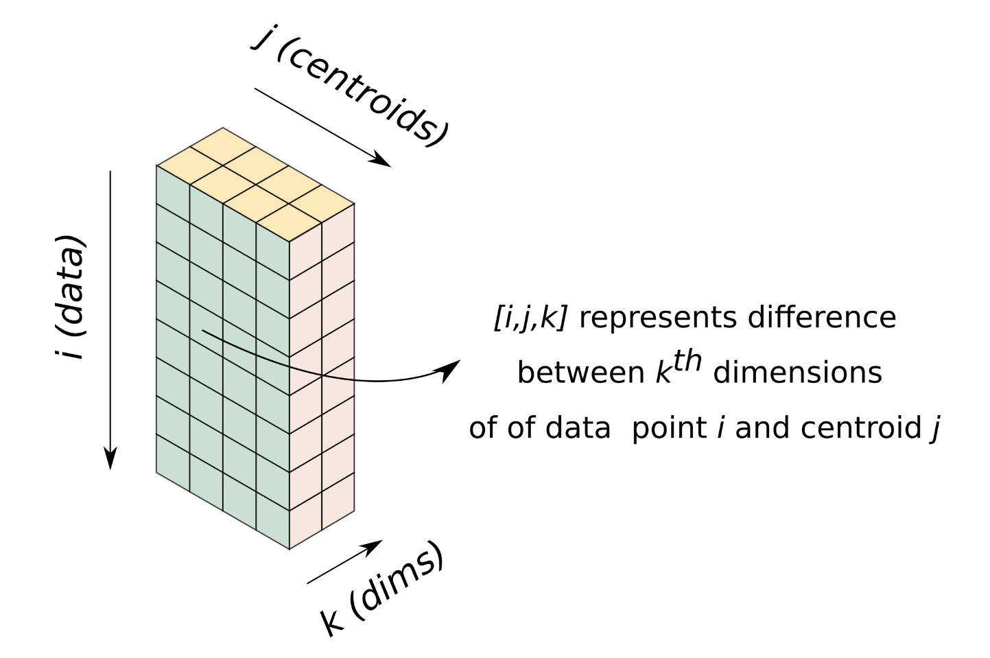
Operating on this array enables us to perform one iteration of K-Means without a loop, enabling us to get rid of the loop over data.
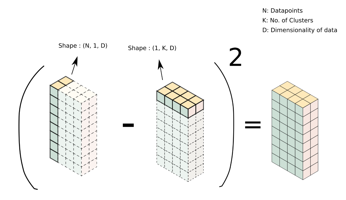
Such an array can be easily created using broadcasting. We have our data as a [4000, 3] array and a centroids as a [4,3] array. To broadcast them, we can reshape data and centroids to [4000, 1, 3] and [1, 4, 3] respectively. Passing these resized arrays to compute_l2_distance results in the formation of the array we talked about above, with the shape [4000, 4, 3].
This can be done simply as:
closest_centroids = get_closest_centroid(data[:, None, :], centroids[None,:, :])
Now that we are dealing with 3-D data and centroid arrays, we must make minor modifications to the helper functions (the axis along which sum and min has to be computed).
def compute_l2_distance(x, centroid):
    # Compute the difference, following by raising to power 2 and summing
    dist = ((x - centroid) ** 2).sum(axis = 2)   # change of axis

    return dist

def get_closest_centroid(x, centroids):

    # Loop over each centroid and compute the distance from data point.
    dist = compute_l2_distance(x, centroids)

    # Get the index of the centroid with the smallest distance to the data point
    closest_centroid_index =  np.argmin(dist, axis = 1) # change of axis

    return closest_centroid_index
Once this is done, we can write our main code without the loop going over dataset.
# Number of dimensions in centroid
num_centroid_dims = data.shape[1]

# List to store SSE for each iteration
sse_list = []

# Main Loop
for n in range(50):
    # Get closest centroids to each data point
    assigned_centroids = get_closest_centroid(data[:, None, :], centroids[None,:, :])

    # Compute new centroids
    for c in range(centroids.shape[1]):
        # Get data points belonging to each cluster
        cluster_members = data[assigned_centroids == c]

        # Compute the mean of the clusters
        cluster_members = cluster_members.mean(axis = 0)

        # Update the centroids
        centroids[c] = cluster_members

    # Compute SSE
    sse = compute_sse(data.squeeze(), centroids.squeeze(), assigned_centroids)
    sse_list.append(sse)
The full entire code can be found here:
Timing the code
Let's time the code now. Using the time module, we get an estimated running time of 0.00073 seconds (+/- 0.00002 seconds) per iteration! Now that's a speed up of 72x for the optimized code!
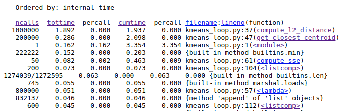
Looking the profiler log of the code:
We see that compute_l2_distance is now only called 100 times, and hence the tottime decreases considerably. get_closest_centroids is only called 50 times and is further down the list.
Conclusion
That brings us to the end of this post! If you were to take anything from this post, it is that merely vectorizing code is not enough; we must also look at which loops have the largest number of iterations. This reminds me of the famous line from George Orwell's Animal Farm:

For loops that have a small number of iterations, you can even leave them be to improve code readability. Of course, there is a trade-off in this case between optimization and readability. That is something I plan to discuss in the future parts of this series, along with concepts like in-place ops, reshaping, transposing, and other options beyond NumPy. Until then, I'll leave you with this key take away message from this post.