Building sharp regression models with K-Means Clustering + SVR

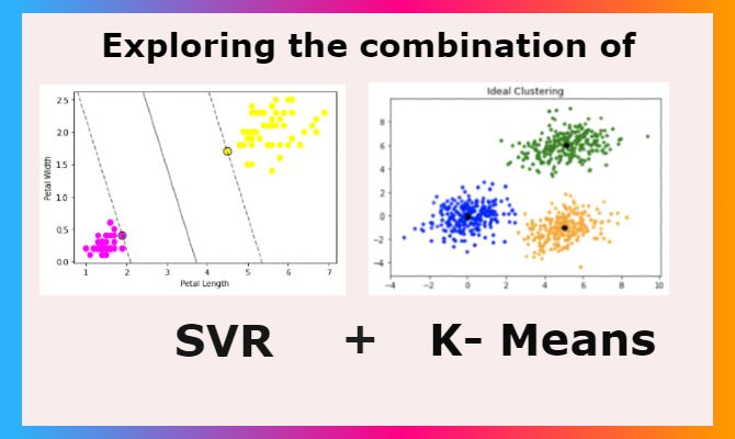
Machine Learning algorithms are diverse in terms of architecture and use cases. One of the most common problems we deal with in Machine Learning is regression, and sometimes regression analyses grow in complexity to the point that existing algorithms fail to predict values with great enough accuracy to be deployed to production. This article dives deep into regression models and how a combination of K-Means and Support Vector Regression can bring up a sharp regression model in certain cases.

Overview

• Regression
• Linear Regression
• Why Linear Regression Fails
• Alternatives
• Support Vector Regression
• K-Means Clustering
• K-Means + SVR Implementation
• Conclusion

Regression

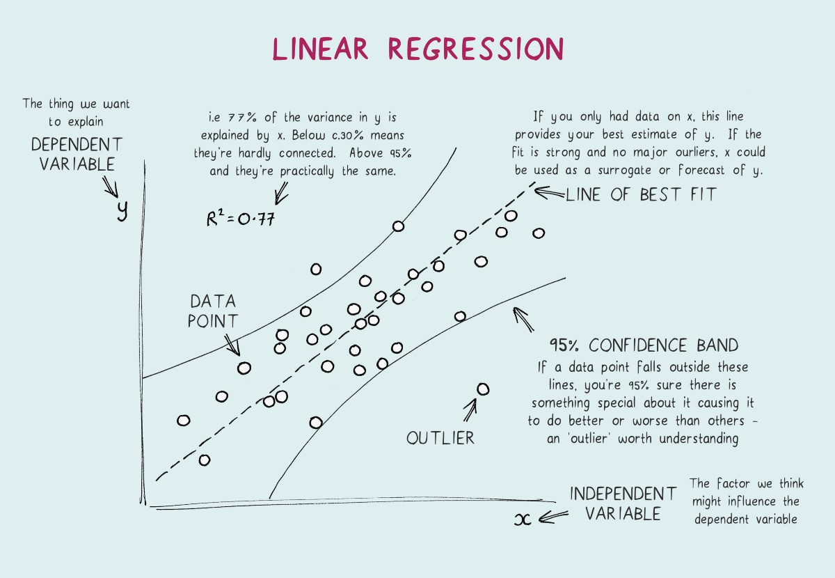
A statistical method used to predict a dependent variable (Y) using certain independent variables (X1, X2,..Xn). In simpler terms, we predict a value based on factors that affect it.

One of the best examples can be an online rate for a cab ride. If we look into the factors that play a role in predicting the price, they are distance, weather, day, area, vehicle, fuel price, and the list goes on. It is difficult to come up with an equation that provides the rate of the ride because of these many factors playing a huge role in it. Regression comes to the rescue by identifying how much each feature as we may call them in Machine Learning terms affect and come up with a model that can predict the rate of a ride. Now that we have got the idea behind regression let's look at Linear Regression.

Linear Regression

Linear regression is the gateway regression algorithm that aims at building a model that tries to find a linear relationship between independent variables (X) and the dependent variable (Y) which is to be predicted. From a visual point of view, we try to create a line such that points are at least distances from it compared to all the other lines possible. Linear regression can handle only one independent variable, but the extension of linear regression, Multiple regression follows the same idea with multiple independent variables contributing to predict the Y. Detailed implementation of Linear Regression.

Why does Linear Regression fail?

Even though linear regression is computationally simple and highly interpretable, it has its own share of disadvantages. It is only preferred when the data is linearly separable. Complex relations cannot be handled by this. A group of data points clustered at one region can highly influence the model and a possible bias will occur. Now that we have understood what regression is and how the basic one works, let's dive deep into some of the alternatives.

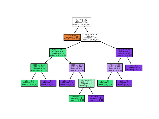
Decision Tree

A decision tree is a tree where each node represents a feature, each branch represents a decision. Outcome (numerical value for regression) is represented by each leaf. Decision trees are capable of capturing non-linear interaction between the features and the target variable. decision trees are easy to understand and interpret. One of the major features is that they are visually intuitive. They are also capable of working with numerical and categorical features.

Some of the cons of using decision trees are that it tends to overfit. Even a small change in the data can cause instability because of the drastic change that might occur to the tree structure in the process.

Random Forest Regression

Random Forest is a combination of multiple decision trees working towards the same objective. Each of the trees is trained with a random selection of the data with replacement, and each split is limited to a variable k features randomly selected with replacement on which to separate the data.

This algorithm works better than a single decision tree in most cases. With multiple trees under the hood, the variations actually help in dealing with new data without any biases. Effectively, this allows a strong learner to be created from a collection of very weak learners. The final regression value is the mean of all the decision trees' outcomes. With huge trees inside it comes with certain downsides such as slow execution while trying to achieve higher performance with all the trees. It also accounts for a huge memory requirement.

Support Vector Regression

Now that we have explored most of the regression algorithms out there, let's explore the one we are focusing on in this article.  Support Vector Regression (SVR) is one of the best regression algorithms that focuses on handling overall error and tries to avoid outlier issues better than algorithms like linear regression. We should first get a good idea about what Support Vector Machines are before we learn about SVR as the idea is derived from there.

Support Vector Machine

The objective of the Support Vector Machine is to come up with a hyperplane in an N-Dimensional vector space, where N is the number of features involved. This hyperplane is expected to classify the data points we provide. It is a great classification algorithm and it works better than logistic regression in many cases because of the hyperplane that keeps data points far apart compared to just a thin line acting as a border. The idea here is to keep data points on either side of the plane, and the ones that fall inside the plane are the outliers here.

The kernel is the major factor behind the performance of the Support Vector Machine that works on dimensionality reduction thereby transforming it into a linear equation. It also succeeds in scaling relatively well to high-dimensional data. The inner product between two points in a standard feature is returned by the kernel. There are different types of kernel functions in SVM.

Gaussian Kernel is used to perform transformation when there is no prior knowledge about data. When data is linearly separable, Linear Kernel is used. The similarity of vectors in the training set of data in a feature space over the polynomials of the original variables used in the kernel is represented by Polynomial Kernel. These are some of the popular kernels and there are more to explore and experiment with. Let's see a small implementation of SVM and visualization of the hyperplane using the Famous Iris dataset.

import seaborn as sns
from sklearn.svm import SVC 
import matplotlib.pyplot as plt
import numpy as np

# Creating dataframe to work on
iris = sns.load_dataset("iris")
y = iris.species
X = iris.drop('species',axis=1)
df=iris[(iris['species']!='versicolor')]
df=df.drop(['sepal_length','sepal_width'], axis=1)

# Converting categorical vlaues to numericals
df=df.replace('setosa', 0)
df=df.replace('virginica', 1)

# Defining features and targer
X=df.iloc[:,0:2]
y=df['species']

# Building SVM Model using sklearn
model = SVC(kernel='linear', C=1E10)
model.fit(X, y)

# plotting the hyperplane created and the data points' distribution
ax = plt.gca()
plt.scatter(X.iloc[:, 0], X.iloc[:, 1], c=y, s=50, cmap='spring')
ax.set(xlabel = "Petal Length",
       ylabel = "Petal Width")
xlim = ax.get_xlim()
ylim = ax.get_ylim()

xx = np.linspace(xlim[0], xlim[1], 30)
yy = np.linspace(ylim[0], ylim[1], 30)
YY, XX = np.meshgrid(yy, xx)
xy = np.vstack([XX.ravel(), YY.ravel()]).T
Z = model.decision_function(xy).reshape(XX.shape)

ax.contour(XX, YY, Z, colors='k', levels=[-1, 0, 1], alpha=0.5,
           linestyles=['--', '-', '--'])

ax.scatter(model.support_vectors_[:, 0], model.support_vectors_[:, 1], s=100,
           linewidth=1, facecolors='none', edgecolors='k')
plt.show()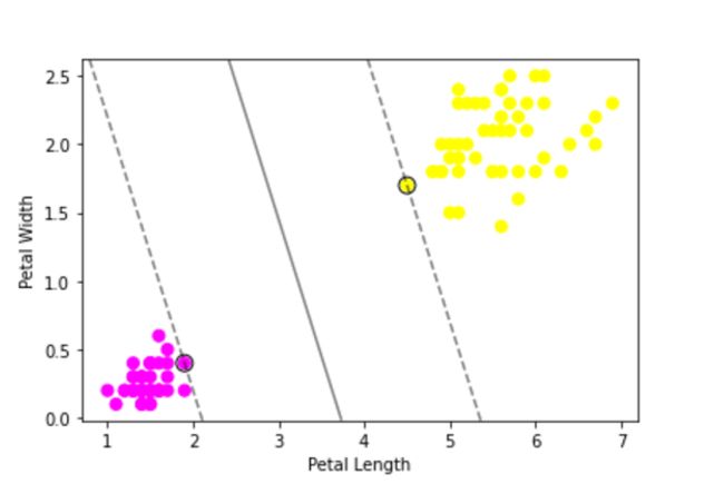

Understanding SVR

Support Vector Regression uses the same principle behind Support Vector Machine. SVR also builds a hyperplane in an N-Dimensional vector space, where N is the number of features involved. Instead of keeping data points away from the hyperplane, here we aim to keep data points inside the hyperplane for regression. One of the tunable parameters is ε (epsilon), which is the width of the tube we create in the feature space. The next regularization parameter that we hypertune is C which controls the "slack" (ξ ) that measures the distance to points outside the tube. Let's see a simple implementation and visualization of SVR before we begin the combination of K-Means clustering and SVR. Here we are using the Real estate price dataset from Kaggle.

import pandas as pd
import numpy as np
from sklearn.svm import SVR # for building support vector regression model
import plotly.graph_objects as go # for data visualization
import plotly.express as px # for data visualization

# Read data into a dataframe
df = pd.read_csv('Real estate.csv', encoding='utf-8')
X=df['X2 house age'].values.reshape(-1,1)
y=df['Y house price of unit area'].values

# Building SVR Model
model = SVR(kernel='rbf', C=1000, epsilon=1) # set kernel and hyperparameters
svr = model.fit(X, y)

x_range = np.linspace(X.min(), X.max(), 100)
y_svr = model.predict(x_range.reshape(-1, 1))

plt = px.scatter(df, x=df['X2 house age'], y=df['Y house price of unit area'], 
                 opacity=0.8, color_discrete_sequence=['black'])

# Add SVR Hyperplane
plt.add_traces(go.Scatter(x=x_range,
	y=y_svr, name='Support Vector Regression', line=dict(color='blue')))
plt.add_traces(go.Scatter(x=x_range,
	y=y_svr+10, name='+epsilon', line=dict(color='blue', dash='dot')))
plt.add_traces(go.Scatter(x=x_range,
	y=y_svr-10, name='-epsilon', line=dict(color='blue', dash='dot')))

# Set chart background color
plt.update_layout(dict(plot_bgcolor = 'white'))

# Updating axes lines
plt.update_xaxes(showgrid=True, gridwidth=1, gridcolor='lightgrey', 
                 zeroline=True, zerolinewidth=1, zerolinecolor='lightgrey', 
                 showline=True, linewidth=1, linecolor='black')

plt.update_yaxes(showgrid=True, gridwidth=1, gridcolor='lightgrey', 
                 zeroline=True, zerolinewidth=1, zerolinecolor='lightgrey', 
                 showline=True, linewidth=1, linecolor='black')

# Update marker size
plt.update_traces(marker=dict(size=3))

plt.show()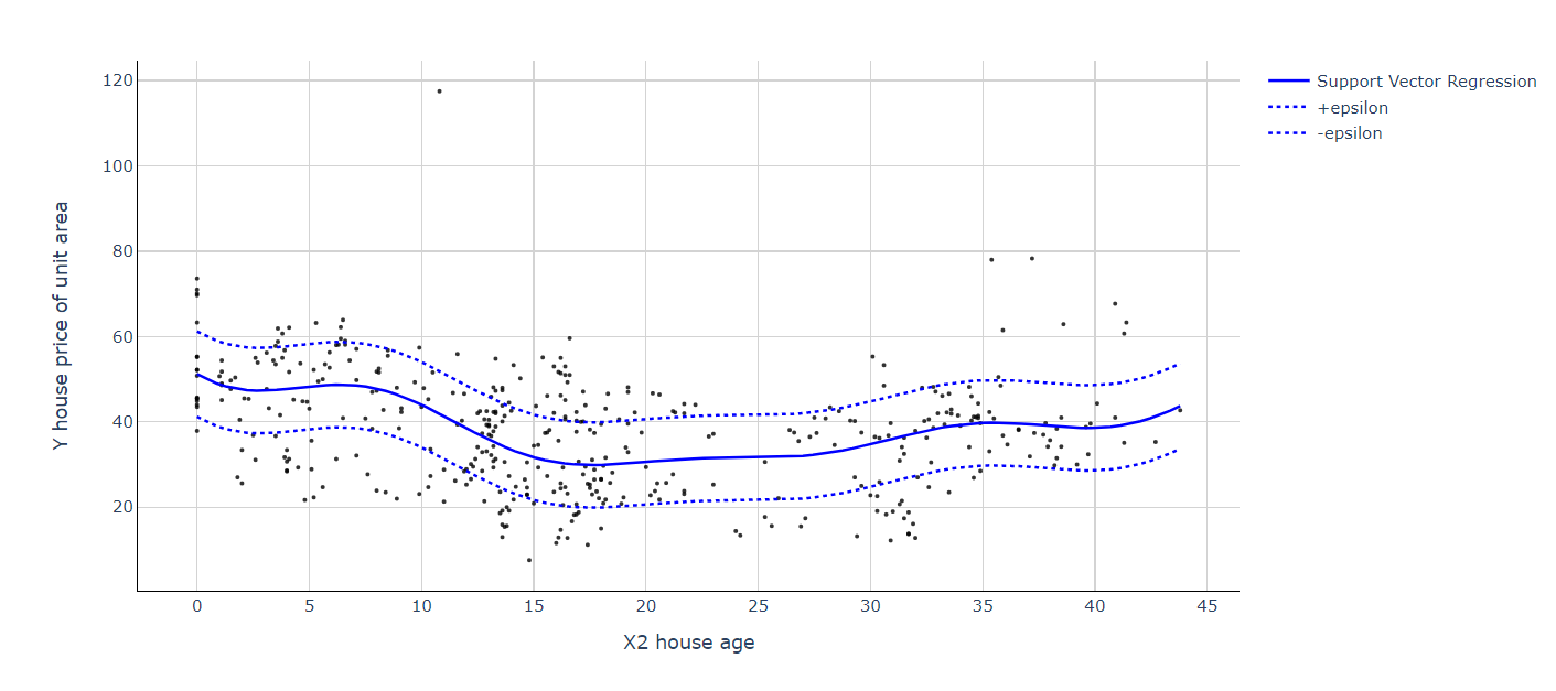

Here we can see that despite the non-linear distribution of data points, SVR neatly handled it with the hyperplane. This effect is even more apparent when we have more than one feature compared to other regression algorithms. Now that we have got a good introduction to SVR, let's explore the amazing combination of K-Means + SVR that can create wonders under the right regression circumstances.

K-Means Clustering

K-Means clustering is a popular unsupervised machine learning algorithm for clustering data. The algorithm works as follows to cluster data points:

• First, we define a number of clusters, let it be K here
• Randomly choose K data points as centroids of the clusters
• Classify data based on Euclidean distance to either of the clusters
• Update the centroids in each cluster by taking means of data points
• Repeat the steps from step 3 for a set number of times (hyperparameter: max_iter)

Even though this seems pretty simple, there are a lot of ways to hypertune K-Means clustering. This includes correctly choosing the points to initialize centroids and a lot more. We will discuss one of them below, the Silhouette Coefficient, which gives a good idea of how many clusters to choose from.

Implementing K-Means Clustering + SVR

We will be using the same Real estate price dataset from Kaggle for this implementation. Here our independent variables are 'X3 distance to the nearest MRT station' and 'X2 house age'.  'Y house price of unit area' is our target variable which we will predict on. Let us first visualize the data points to define the need for clustering.

import pandas as pd # for data manipulation
import numpy as np # for data manipulation
import matplotlib.pyplot as plt

# Read data into a dataframe
df = pd.read_csv('Real estate.csv', encoding='utf-8')

# Defining Dependent and Independant variable
X = np.array(df[['X3 distance to the nearest MRT station','X2 house age']])
Y = df['Y house price of unit area'].values

# Plotting the Clusters using matplotlib
plt.rcParams['figure.figsize'] = [14, 7]
plt.rc('font', size=14)

plt.scatter(df['X3 distance to the nearest MRT station'],df['X2 house age'],label="cluster "+ str(i+1))
plt.xlabel("X3 distance to the nearest MRT station")
plt.ylabel("X2 house age")
plt.legend()
plt.show()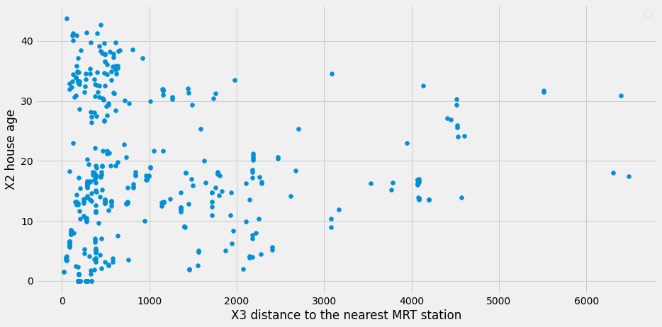

Clearly, data points are not having a good distribution to suit a hyperplane that contains them. Let us cluster them using K-Means clustering. Before we start, we can use the Silhouette Coefficient to determine the number of clusters we need that can keep data points accurately in the selected number of clusters. Better Silhouette Coefficient or Score means better clustering. It signifies the distance between the clusters. A maximum score of 1 implying clusters are well apart from each other and also clearly distinguished, a score of 0 implying insignificant distance between the clusters, and -1 implying incorrect assigning of clusters.

Let us first evaluate Silhouette Coefficient for our data points. We will split data into train and test from here to start moving towards our final objective. Clustering will be executed over the training data.

from sklearn.model_selection import train_test_split
from sklearn.cluster import KMeans
from sklearn.metrics import silhouette_score
import statistics
from scipy import stats

X_train, X_test, Y_train, Y_test = train_test_split(
 X, Y, test_size=0.30, random_state=42)

silhouette_coefficients = []

kmeans_kwargs= {
    "init":"random",
    "n_init":10,
    "max_iter":300,
    "random_state":42
}

for k in range(2, 11):
    kmeans = KMeans(n_clusters=k, **kmeans_kwargs)
    kmeans.fit(X_train)
    score = silhouette_score(X_train, kmeans.labels_)
    silhouette_coefficients.append(score)
    
# Plotting graph to choose the best number of clusters
# with the most Silhouette Coefficient score

import matplotlib.pyplot as plt

plt.style.use("fivethirtyeight")
plt.plot(range(2, 11), silhouette_coefficients)
plt.xticks(range(2, 11))
plt.xlabel("Number of Clusters")
plt.ylabel("Silhouette Coefficient")
plt.show()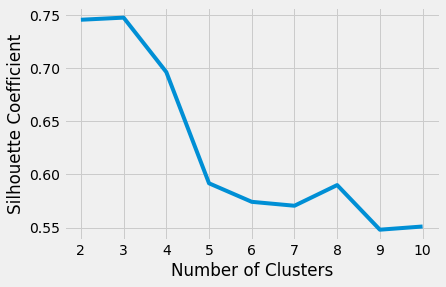

We can arrive at the conclusion that with 3 clusters, we can achieve better clustering. Let's go ahead and cluster the training set data.

from sklearn.cluster import KMeans
import matplotlib.pyplot as plt
import pandas as pd # for data manipulation
import numpy as np # for data manipulation

# Instantiate the model: KMeans from sklearn
kmeans = KMeans(
    init="random",
    n_clusters=3,
    n_init=10,
    max_iter=300,
    random_state=42
)

# Fit to the training data
kmeans.fit(X_train)

train_df = pd.DataFrame(X_train,columns=['X3 distance to the nearest MRT station','X2 house age'])

# Generate out clusters
train_cluster = kmeans.predict(X_train)

# Add the target and predicted clusters to our training DataFrame
train_df.insert(2,'Y house price of unit area',Y_train) 
train_df.insert(3,'cluster',train_cluster) 
n_clusters=3
train_clusters_df = []
for i in range(n_clusters):
    train_clusters_df.append(train_df[train_df['cluster']==i])
    
colors = ['red','green','blue']
plt.rcParams['figure.figsize'] = [14, 7]
plt.rc('font', size=12)

# Plot X_train again with features labeled by cluster
for i in range(n_clusters):
  subset = []
  for count,row in enumerate(X_train):
      if(train_cluster[count]==i):
        subset.append(row)

  x = [row[0] for row in subset]
  y = [row[1] for row in subset]
  plt.scatter(x,y,c=colors[i],label="cluster "+ str(i+1))
plt.title("Train Data Clusters", x=0.6, y=0.95)
plt.xlabel("X3 distance to the nearest MRT station")
plt.ylabel("X2 house age")
plt.legend()
plt.show()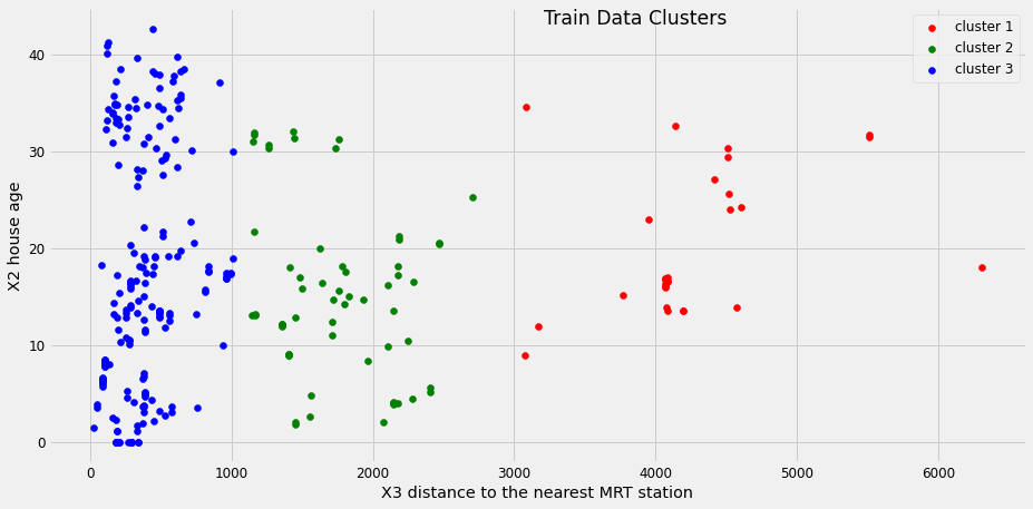

Building SVR for clusters

Now, let us go ahead and build SVR Models for each cluster. We are not focusing on the hypertuning of SVR's here. It can be done if needed by trying out various combinations of parameter values using a gridsearch.

import pandas as pd
import numpy as np
from sklearn.svm import SVR

n_clusters=3
cluster_svr = []
model = SVR(kernel='rbf', C=1000, epsilon=1)

for i in range(n_clusters):
    cluster_X = np.array((train_clusters_df[i])[['X3 distance to the nearest MRT station','X2 house age']])
    cluster_Y = (train_clusters_df[i])['Y house price of unit area'].values
    cluster_svr.append(model.fit(cluster_X, cluster_Y))

Let us define a function that will predict House Price (Y) by predicting the cluster first, and then the value with the corresponding SVR.

def regression_function(arr, kmeans, cluster_svr):
    result = []
    clusters_pred = kmeans.predict(arr)
    for i,data in enumerate(arr):
        result.append(((cluster_svr[clusters_pred[i]]).predict([data]))[0])
    return result,clusters

Now that we have built our end-to-end flow for prediction and constructed the required models, we can go ahead and try this out on our test data. Let us first visualize the clusters of test data with the K means cluster we built, and then find the Y value using the corresponding SVR using the function we have written above.  

from sklearn.cluster import KMeans
import matplotlib.pyplot as plt

# calculating Y value and cluster
Y_svr_k_means_pred, Y_clusters = regression_function(X_test,
	kmeans, cluster_svr)
    
colors = ['red','green','blue']
plt.rcParams['figure.figsize'] = [14, 7]
plt.rc('font', size=12)

n_clusters=3

# Apply our model to clustering the remaining test set for validation

for i in range(n_clusters):
  subset = []
  for count,row in enumerate(X_test):
      if(Y_clusters[count]==i):
        subset.append(row)

  x = [row[0] for row in subset]
  y = [row[1] for row in subset]
  plt.scatter(x,y,c=colors[i],label="cluster "+ str(i+1))
plt.title("Test Data Clusters", x=0.6, y=0.95)
plt.xlabel("X3 distance to the nearest MRT station")
plt.ylabel("X2 house age")
plt.legend()
plt.show()

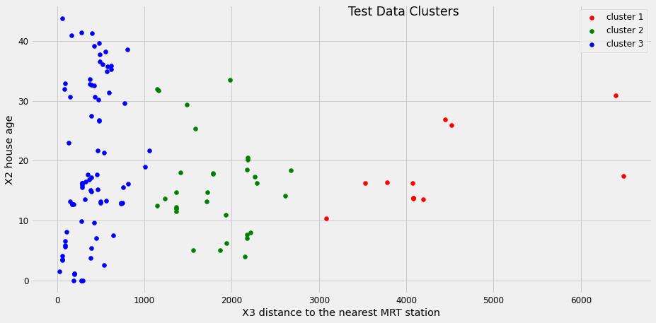
We can clearly see that we have got definite clusters for test data, and, also, got the Y value and have been stored in Y_svr_k_means_pred. Let us store the results and data into a data frame along with the cluster.

import pandas as pd

result_df = pd.DataFrame(X_test,columns=['X3 distance to the nearest MRT station','X2 house age'])
result_df['Y true value'] =  Y_test
result_df['Y SVR + K means'] = Y_svr_k_means_pred
result_df['cluster'] = Y_clusters
result_df.head()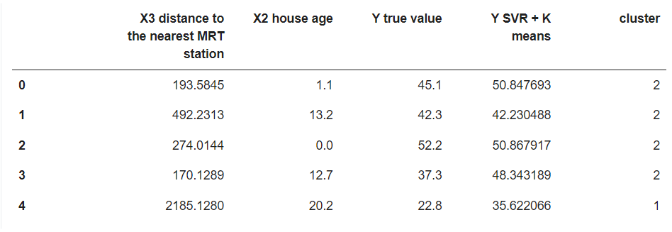

Some of the results are really good and others are still better than what a linear regression or SVR alone model can predict. This was just an example of how to approach such problems and both K means and SVR. This method only performs well when data points are not distributed properly and there is a scope for clustered data handling. This was an example with just two independent variables. If the numbers increase, complexity will also increase, making it difficult to handle such cases with ordinary algorithms, and in such cases, trying this method may help.

The approach we had here was first to visualize the data or evaluate whether there is a chance for clustered handling. Then performing K- Means clustering on the train data. K-Means can be hypertuned using the Silhouette Coefficient score, which will help us get the ideal number of clusters for our problem. After clustering, we build Support Vector Regression for each cluster and the final workflow including all the models we built follows the idea of first predicting the cluster, then predicting the dependent variable (Y) using the corresponding SVR model of that cluster.

Conclusion

Regression is one of the straightforward tasks carried out in Machine Learning. Still, it can become increasingly difficult to find the right algorithm that can build a model with decent accuracy for deploying to production. It is always better to try most of the algorithms out there before finalizing one. There may be instances where a simple linear regression would have worked wonders instead of the huge random forest regression. Having a solid understanding of the data and its nature will help us choose algorithms easily and visualization also helps in the process. This article focuses on exploring the possibility of the combination of K-Means clustering and Support Vector Regression. This approach won't always suit all the cases of regression as it stresses the clustering possibility. One good example of such a problem can be soil moisture prediction as it may vary with seasons and a lot of cyclic features, resulting in clustered data points. K-Means clustering saves us from manual decisions on clusters and SVR handles non-linearity very well. Both SVR and K-Means alone have a lot more in-depth to explore including Kernels, centroid initialization, and the list goes on, so I highly encourage you to read more on the topics to yield a better model. Thanks for reading!