Improving Model Accuracy with Transfer Learning, Data Augmentation, LR Finder, and Much More

It's easy to get more than 90% accuracy when dealing with popular datasets which are cleaned, tested, split and handled beforehand by experts. You just need to import and feed the dataset to the most popular model architecture found on the internet.

In image classification, things get a bit difficult when you are left with a new dataset that has very few images in a class or if the images are not similar to the images you will deal in production. The popular model architecture doesn't seem to help, forcing you into a corner with just 50% accuracy which then turns into a game of probability rather than Machine Learning itself.

This article focuses on exploring all of those approaches, tools, and much more to help you build robust models that can be deployable in production without much hassle. Even though some of the methods are applicable to other objectives too, we are focusing on Image Classification to explore the topic.

Why do Custom Datasets fail in achieving high accuracy?

It is important to address why custom datasets fail mostly in achieving good performance metrics. You might have faced this while trying to use a dataset you created or ones that you got from your team to create a model. Lack of diversity can be one of the main reasons behind the poor performance of the model built on it. Parameters such as lighting, colors, shape, etc of the image can have significant variation, and this may not be considered while constructing the dataset. Data Augmentation might help you solve this, which we will discuss further.

Another reason can be the lack of focus on each category: a dataset with 1000+ images of one type of coffee and just 100+ images of the other creates a big imbalance in the features that could be learned. Another failure can be from the source of data collection not matching the source from where data will be collected in production. A good example of such a situation can be bird detection from a security camera with poor video quality taken as input for a model trained on high-definition images. There are various approaches with which such situations can be tackled.

Why does Production level accuracy matter?

Since we’ve discussed why custom datasets fail to achieve "Production Level Accuracy" on the first run, it is important to understand why Production Level Accuracy matters. Simply put, our models should be able to give results that are adequately acceptable in real-world scenarios,  but not necessarily striving for 100% accuracy. It's easy to see the right predictions with test dataset images or text which was used to hypertune the model to its best. Even though we cannot fix a threshold accuracy above which our model is eligible for deployment, it's good to have at least 85-90% validation accuracy as a rule of thumb, given that train and validation data were split randomly. Always ensure validation data is diverse and that the majority of its data resembles that which the model will consume in production. Data preprocessing can help you achieve this to a certain extent by ensuring the image size by resizing or filtering text before input. Handling such errors during development can help improve your production mode and obtain better results.

Data Augmentation: A perfect way to improve your dataset

It's okay to have a small dataset as long as you can get the best out of it through approaches such as data augmentation. This concept focuses on pre-processing existing data to generate more diverse data for training at times when we don't have enough data. Let us discuss a bit around Image Data Augmentation with a small example. Here we have a rock paper scissors dataset from TensorFlow and we wish to generate more without repeating. Tensorflow dataset objects provide a lot of operations that help in data augmentation and much more. Here we first cache the dataset, which helps us in memory management as the first time the dataset is iterated over, its elements will be cached in the specified file or in memory. Then cached data can be used afterward.

We repeat the dataset twice after that, which increases its cardinality. Just repeated data doesn't help us, but we add a mapping layer over the doubled dataset which in a way helps us generate new data along with the increase in cardinality. In this example, we are flipping random images to left and right which avoids repetition and ensures diversity.

import tensorflow as tf
import tensorflow_datasets as tfds


DATASET_NAME = 'rock_paper_scissors'

(dataset_train_raw, dataset_test_raw), dataset_info = tfds.load(
    name=DATASET_NAME,
    data_dir='tmp',
    with_info=True,
    as_supervised=True,
    split=[tfds.Split.TRAIN, tfds.Split.TEST],
)

def preprocess_img(image, label):
    # Make image color values to be float.
    image = tf.cast(image, tf.float32)
    # Make image color values to be in [0..1] range.
    image = image / 255.
    # Make sure that image has a right size
    image = tf.image.resize(image, [256,256])
    return image, label

dataset_train = dataset_train_raw.map(preprocess_img)
dataset_test = dataset_test_raw.map(preprocess_img)

print("Dataset Cardinality Before Augmentation: ",dataset_train.cardinality().numpy())

dataset_train = dataset_train.cache().repeat(2).map(
    lambda image, label: (tf.image.random_flip_left_right(image), label)
)

print("Dataset Cardinality After Augmentation: ",dataset_train.cardinality().numpy())

Output

Dataset Cardinality Before Augmentation:  2520
Dataset Cardinality After Augmentation:  5040

There are more mappings on images to explore that can further create more variations in terms of contrast, rotation, and much more. Read this article for more details.  There are many more operations you can perform on an image like rotate, shear, vary contrast, and much more. Data augmentation is crucial in cases where image data is not representative of the real-world inputs in terms of lighting, background, and other aspects. Here we discussed data augmentation through frameworks like Tensorflow, but you can do manual data augmentation with much more than rotate and shear.

Mapping is a strong tool because you can perform any operation on individual data without going through iterations. Resizing Images, formatting text, and much more can be handled neatly with this.

Transfer Learning: Working with small datasets

There are situations when you have only a few images and you wish to build an image classification model. With few images, the model might fail to learn patterns and much more, and it will result in an overfit or underfit model that would perform poorly in production with real-world inputs. The easiest way to build a good model in such conditions is through Transfer Learning.

There are famous pre-trained models like VGG16 that are really good at image classification. Because of the wide variety of data it has been exposed to while building, and the complex nature of its architecture (including a lot of convolutional neural networks), it has more depth in the objective of image classification than the small model which we can build with a small dataset. We can use such pre-trained models that deal with the same objective for our problem by just replacing a few of the last layers (in most cases). The reason why we Replace the last layer is to restructure the model output that suits our use case, and select the right number of categories to classify in the case of image classification. We can replace not just the last but as many layers as we wish if we follow the documentation of the respective pre-trained model architecture and the framework documentation around it. Let us build a sample Transfer Learning Machine Learning Model.

First, we are loading and pre-processing the same rock paper scissors dataset we used previously.

import tensorflow as tf
import tensorflow_datasets as tfds
from tensorflow.keras.applications import ResNet50
from keras.layers import GlobalAveragePooling2D, Dense
from keras.layers import BatchNormalization, Dropout
from keras.models import Model

DATASET_NAME = 'rock_paper_scissors'

(dataset_train_raw, dataset_test_raw), dataset_info = tfds.load(
    name=DATASET_NAME,
    data_dir='tmp',
    with_info=True,
    as_supervised=True,
    split=[tfds.Split.TRAIN, tfds.Split.TEST],
)

def preprocess_img(image, label):
    # Make image color values to be float.
    image = tf.cast(image, tf.float32)
    # Make image color values to be in [0..1] range.
    image = image / 255.
    # Resize images to ensure same input size
    image = tf.image.resize(image, [256,256])
    return image, label

dataset_train = dataset_train_raw.map(preprocess_img)
dataset_test = dataset_test_raw.map(preprocess_img)

dataset_train = dataset_train.batch(64)
dataset_test = dataset_test.batch(32)

Now we will use ResNet50 for our transfer learning model. We will set trainable = false to freeze the ResNet50 Architecture and not expose it to training. This will save us a lot of time as the model will train only the last few layers. This is beneficial when we do training on a paid instance on an hourly basis.

# ResNet50 with Input shape of our Images
# Include Top is set to false to allow us to add more layers

res = ResNet50(weights ='imagenet', include_top = False, 
               input_shape = (256, 256, 3)) 
               
# Setting the trainable to false
res.trainable = False


x= res.output
x = GlobalAveragePooling2D()(x)
x = BatchNormalization()(x)
x = Dropout(0.5)(x) 
x = Dense(512, activation ='relu')(x)
x = BatchNormalization()(x)
x = Dropout(0.5)(x)
x = Dense(3, activation ='softmax')(x)
model = Model(res.input, x)

model.compile(optimizer ='Adam', 
              loss ="sparse_categorical_crossentropy", 
              metrics =["sparse_categorical_accuracy"])

model.summary()

Model Summary in short

( Only the Bottom part of Model Summary Included here as the ResNet Summary is long)
_____________________________________________________________________________
conv5_block3_out (Activation)   (None, 8, 8, 2048)   0           conv5_block3_add[0][0]           
_____________________________________________________________________________
global_average_pooling2d_5 (Glo (None, 2048)         0           conv5_block3_out[0][0]           
_____________________________________________________________________________
batch_normalization_11 (BatchNo (None, 2048)         8192        global_average_pooling2d_5[0][0] 
_____________________________________________________________________________
dropout_11 (Dropout)            (None, 2048)         0           batch_normalization_11[0][0]     
_____________________________________________________________________________
dense_11 (Dense)                (None, 512)          1049088     dropout_11[0][0]                 
_____________________________________________________________________________
batch_normalization_12 (BatchNo (None, 512)          2048        dense_11[0][0]                   
_____________________________________________________________________________
dropout_12 (Dropout)            (None, 512)          0           batch_normalization_12[0][0]     
_____________________________________________________________________________
dense_12 (Dense)                (None, 3)            1539        dropout_12[0][0]                 
=============================================================================
Total params: 24,648,579
Trainable params: 1,055,747
Non-trainable params: 23,592,832

Model Training

model.fit(dataset_train, epochs=6, validation_data=dataset_test)

Epoch 1/10
40/40 [==============================] - 577s 14s/step - loss: 0.2584 - sparse_categorical_accuracy: 0.9147 - val_loss: 1.1330 - val_sparse_categorical_accuracy: 0.4220

Epoch 2/10
40/40 [==============================] - 571s 14s/step - loss: 0.0646 - sparse_categorical_accuracy: 0.9802 - val_loss: 0.8574 - val_sparse_categorical_accuracy: 0.4247

Epoch 3/10
40/40 [==============================] - 571s 14s/step - loss: 0.0524 - sparse_categorical_accuracy: 0.9813 - val_loss: 0.7408 - val_sparse_categorical_accuracy: 0.6425

Epoch 4/10
40/40 [==============================] - 570s 14s/step - loss: 0.0376 - sparse_categorical_accuracy: 0.9881 - val_loss: 0.6260 - val_sparse_categorical_accuracy: 0.7016

Epoch 5/10
40/40 [==============================] - 570s 14s/step - loss: 0.0358 - sparse_categorical_accuracy: 0.9881 - val_loss: 0.5864 - val_sparse_categorical_accuracy: 0.6532

Epoch 6/10
40/40 [==============================] - 570s 14s/step - loss: 0.0366 - sparse_categorical_accuracy: 0.9873 - val_loss: 0.4445 - val_sparse_categorical_accuracy: 0.8602

We can see how a model trained on a relatively small dataset performed very well with a validation accuracy of 86%. If you focus on the time taken for each epoch, it's less than 10 minutes, as we kept the ResNet layers not trainable. ResNet50 helped us transfer its learning to our problem. You can experiment with various Pre-trained Models to see how they suit your problem and which perform best.

LR Finder: Finding the perfect Learning Rate

Learning Rate Finder is a powerful tool that can help you find the LR as the name suggests easily. Trying out all the learning rates to find the perfect learning rate is an inefficient and time-consuming method. LR Finder is the efficient and least time-consuming way to do this. Let's see how to implement it. We are continuing with the same dataset, preprocessing and model architecture, so it's not repeated from here on.

!pip install tensorflow-hub
!git clone https://github.com/beringresearch/lrfinder/
!cd lrfinder && python3 -m pip install .

import numpy as np
from lrfinder import LRFinder
K = tf.keras.backend

BATCH = 64

# STEPS_PER_EPOCH = np.ceil(len(train_data) / BATCH)
# here Cardinality or Length of Train dataset is 2520


STEPS_PER_EPOCH = np.ceil(2520 / BATCH)
lr_finder = LRFinder(model)
lr_finder.find(dataset_train, start_lr=1e-6, end_lr=1, epochs=10,
               steps_per_epoch=STEPS_PER_EPOCH)
               
learning_rates = lr_finder.get_learning_rates()
losses = lr_finder.get_losses()

best_lr = lr_finder.get_best_lr(sma=20)

# Setting it as our model's LR through Keras Backend
K.set_value(model.optimizer.lr, best_lr)
print(best_lr)

Epoch 1/10
40/40 [==============================] - 506s 13s/step - loss: 1.7503 - sparse_categorical_accuracy: 0.3639
Epoch 2/10
40/40 [==============================] - 499s 12s/step - loss: 1.5044 - sparse_categorical_accuracy: 0.4302
Epoch 3/10
40/40 [==============================] - 498s 12s/step - loss: 0.9737 - sparse_categorical_accuracy: 0.6163
Epoch 4/10
40/40 [==============================] - 495s 12s/step - loss: 0.4744 - sparse_categorical_accuracy: 0.8218
Epoch 5/10
40/40 [==============================] - 495s 12s/step - loss: 0.1946 - sparse_categorical_accuracy: 0.9313
Epoch 6/10
40/40 [==============================] - 495s 12s/step - loss: 0.1051 - sparse_categorical_accuracy: 0.9663
Epoch 7/10
40/40 [==============================] - 89s 2s/step - loss: 0.1114 - sparse_categorical_accuracy: 0.9576

The best Learning Rate we get is 6.31 e-05, and we set it as our LR for the model using Keras Backend. From the Outputs, it's clear that this process took only a few epochs and it analyzed all the possible learning rates and found the best one. We can visualize the learning rates and their performance using Matplotlib. The red line represents the best learning rate.

import matplotlib.pyplot as plt

def plot_loss(learning_rates, losses, n_skip_beginning=10, n_skip_end=5, x_scale='log'):
    f, ax = plt.subplots()
    ax.set_ylabel("loss")
    ax.set_xlabel("learning rate (log scale)")
    ax.plot(learning_rates[:-1],
            losses[:-1])
    ax.set_xscale(x_scale)
    return(ax)

axs = plot_loss(learning_rates, losses)
axs.axvline(x=lr_finder.get_best_lr(sma=20), c='r', linestyle='-.')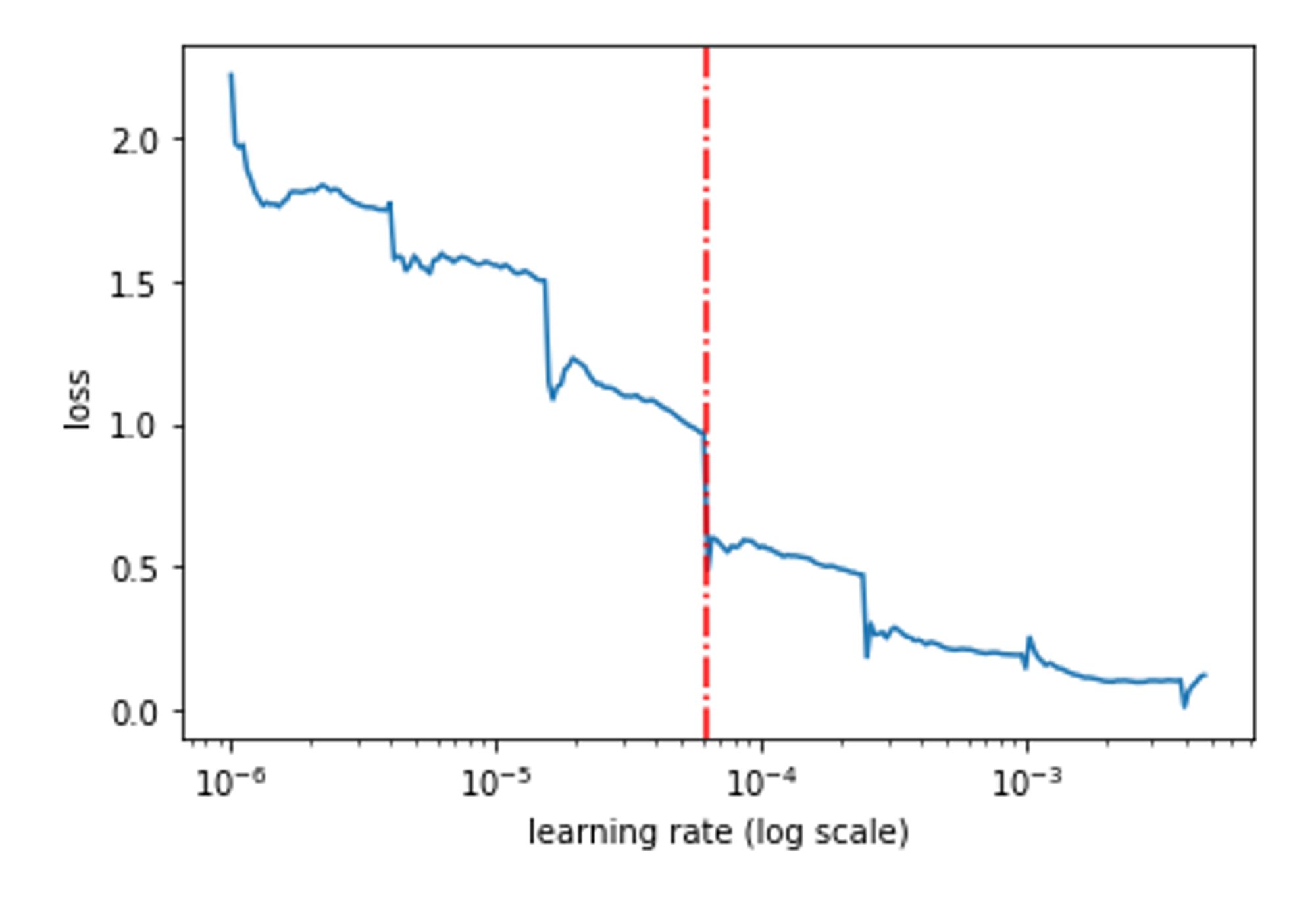

Early Stopping: Rescuing your model before it unlearns

You might remember training a model for 20+ epochs, and the model's loss starts to increase after a point.  You're stuck, and you can't do anything as interrupting will kill the process, and waiting will give you a more poorly performing model. Early Stopping is exactly what you want in such situations where you can easily secure your best model and escape the process once parameter like loss starts increasing. This will save you time also as if the model starts showing positive loss early, the process will be stopped by providing you with the last best loss model and not computing further epochs. You can set early stopping based on any able to be monitored parameter like accuracy, as well. One of the major parameters of early stopping is patience. It is the number of epochs you wish to see if the model stops showing an increased loss and gets back to the track of learning, or else it will save the last best loss before the increase and stop the training. Now that you might have got a small idea, let's jump into an example.

from tensorflow.keras.callbacks import EarlyStopping

earlystop_callback = EarlyStopping(
  monitor='val_loss', min_delta=0.0001, patience=2)

model.fit(dataset_train, epochs=20, validation_data=dataset_test, callbacks=[earlystop_callback])

In the example, early stopping is set to monitor validation loss. The parameter minimum delta, which is the minimum difference we want in loss, is set to 0.0001, and patience is set to 2. A patience of 2 implies that the model can go for 2 more epochs with increased validation loss, but if it doesn't show a decreased loss then (lower than the loss from where it started to increase) the process will be killed by returning the last best loss version.

( Only the last part of training shown )

Epoch 10/20
40/40 [==============================]  loss: 0.0881 - sparse_categorical_accuracy: 0.9710 - val_loss: 0.4059 
Epoch 11/20
40/40 [==============================]  loss: 0.0825 - sparse_categorical_accuracy: 0.9706 - val_loss: 0.4107 
Epoch 12/20
40/40 [==============================]  loss: 0.0758 - sparse_categorical_accuracy: 0.9770 - val_loss: 0.3681 
Epoch 13/20
40/40 [==============================]  loss: 0.0788 - sparse_categorical_accuracy: 0.9754 - val_loss: 0.3904 
Epoch 14/20
40/40 [==============================]  loss: 0.0726 - sparse_categorical_accuracy: 0.9770 - val_loss: 0.3169 
Epoch 15/20
40/40 [==============================]  loss: 0.0658 - sparse_categorical_accuracy: 0.9786 - val_loss: 0.3422 
Epoch 16/20
40/40 [==============================]  loss: 0.0619 - sparse_categorical_accuracy: 0.9817 - val_loss: 0.3233 

Even with 20 epochs set to train, the model stopped training after the 16th epoch saving the model from unlearning with increased validation loss. Our training results have some really good observations that can help us get a deeper understanding of early stopping.  On 14th epoch model was at its best loss, 0.3168. The next epoch showed an increased loss of 0.3422 and even though the following epoch showed a decreased loss of 0.3233 which is less than the previous, it's still larger than the point from where the increase started (0.3168), so training stopped with the model version at 14th epoch saved. It waited for 2 epochs to see if the training would correct itself because of the patience parameter being set to 2.

Another interesting observation is from the 10th to 12th epoch, even though the loss increased on the 11th epoch (0.4107), the 12th epoch showed a decreased loss (0.3681) compared to the 10th epoch's (0.4059). Thus training continued as the model got back to track. This can be treated as a good use of patience as leaving it to default would have killed the training after the 11th epoch, not trying for the next one.

Some tips on using early stopping are that if you are training on CPU, use a small patience setting. if training on GPU, use larger patience values. For models like GAN, it's better to use small patience and save model checkpoints. If your dataset doesn't contain large variations, then use larger patience. Set the min_delta parameter always based on running few epochs and checking validation loss, as this will give you an idea of how your validation loss is varying from epoch to epoch.

Analyzing your Model architecture

This is a general approach rather than a definitive one. In most cases such as Image classifications which involve Convolutional Neural Networks, it is really important that you are well aware of your convolutions, their kernel size, output shape, and much more even though frameworks handle the flow. Very deep architectures like ResNet are made to train on 256x256 sized images, and resizing it to fit your case where the dataset images are 64x64 might perform so poorly it results in accuracies of 10% for certain pre-trained models. This is because of the number of layers in the pre-trained models and your image size. As it is clear that image tensors become smaller in terms of size as they go through convolutions, as the channels increase in parallel. A pre-trained model trained on 256x256 will have a tensor size of at least 8x8 by the end whereas if you restructure it for 64x64, the last few convolutions will get 1x1 tensors which learn very little compared to an 8x8 input. This is something to be handled carefully when handling pre-trained models.

The other side of this is when you build your own convolutions. Make sure it has some depth with more than 3 layers, and, at the same time, it also doesn't affect the output size considering your image size. Analyzing the model summary is really important, as you can decide on setting your Dense layers based on the output shape of the convolutional layer and much more. While dealing with Multiple Features and Multiple Outputs models, architecture matters a lot. In such cases, Model Visualization helps.

Conclusion

So far we have discussed some of the most impactful and popular approaches that can improve your model accuracy, improve your dataset, and better your model architecture. There are plenty of other ways out there for you to explore. Along with these, there are more minor approaches or guidelines that can help you achieve all the above aspects such as shuffling while data loading, using TensorFlow dataset object to work on your custom-created dataset, using mapping as we discussed earlier to handle operations. I recommend you focus on Validation accuracy while training rather than training accuracy. Validation Data must be treated very well, and its diversity and representative nature to the real-world input the model will be exposed to in production is significant.

Even though we performed all the approaches on an Image Classification problem, some of them like mapping, learning rate finder, etc. are applicable to other problems involving text and much more. Building a model with below-average accuracy is not valuable in real life as accuracy matters and in such situations, these approaches can help us build a model close to perfection with all the aspects taken care of. One of the popular approaches, Hyperparameter tuning is not discussed in this article in detail. It is in short trying out various values for Hyperparameters such as epochs, batch size, etc. The aim of Hyperparameter tuning is to achieve the best parameters and eventually getting a better model. LR Finder is an efficient way of hyperparameter tuning the Learning Rate. When dealing with other Machine Learning algorithms such as SVR, Hyperparameter tuning plays a crucial role.

I hope you have got a good idea on how important it is to work on your model with various ideas and approaches to achieve better performance and all the best for your Machine Learning journey ahead. I hope these approaches come in handy in your way. Thanks for reading!