Image Captioning With TensorFlow And Keras

When we look at an image, our visual perception of that particular image can interpret a lot of different things. For example, in the above image, one of the interpretations by the visual perception in our brain could be "The sailing of a boat with passengers in a river," or we could totally disregard the boat and focus on other elements with an interpretation such as "A beautiful scenery depicting some buildings with a bridge." While none of these perspectives of any provided image are incorrect, sometimes it becomes essential to address the main entity in the image pattern and comment a line about it. The human brain should have no trouble accessing any of the following information on viewing any particular visual patterns. However, is it actually possible for neural networks to uncover such a complex problem and interpret the solution as our human brain with the perfect eye receptors would be able to?

This question is quite intriguing. The solution to such a problem looks to be highly optimistic because, with the right ideas, we can successfully perform the implementation of the previously mentioned tasks. The problem of image captioning is solvable with the combined usage of our two previous articles, namely the "Machine Translation With Sequence To Sequence Models And Dot Attention Mechanism" and "A Complete Intuitive Guide To Transfer Learning." I would highly recommend any readers who haven't already checked out the following two articles to immediately do so if they don't have a piece of complete theoretical knowledge on these two elements. The combined knowledge of transfer learning for analyzing the images and the Sequence to Sequence models with Attention for interpreting the appropriate text data is useful for solving the problem of image captioning.

With a brief introduction and some other smaller intricate details, this guide will dive straight into the contraction of the image captioning project with TensorFlow and Keras. I would highly recommend any beginners to deep learning to check out most of the basic topics without skipping any of the essential concepts. However, if you are comfortable with the project of image captioning, and only want to focus on certain specifics or essentials, the list of the table of contents is provided below. This guide should be able to guide you through the various significant topics that are discussed in this article.

Introduction:

Before we dive straight into the construction of the project, let us understand the concepts of image captioning. So, what exactly is image captioning? Image captioning is a method of generating textual descriptions for any provided visual representation (such as an image or a video). While the process of thinking of appropriate captions or titles for a particular image is not a complicated problem for any human, this case is not the same for deep learning models or machines in general. However, with the right amount of information and datasets, perfect architectural structure builds, and sufficient useful resources, the task of image captioning with fairly high accuracy can be achieved.

The applications of image captioning are extremely numerous in the modern world. To mention a few of the remarkable applications of image captioning, we can include their use cases in recommendations in editing applications, usage in virtual assistants, for image indexing, for visually impaired persons, for social media, and a plethora of other natural language processing applications. It is also overall a fun project to build from scratch with the help of TensorFlow and Keras, but please ensure that your environment meets the requirements for running such a project.

The knowledge of the deep learning frameworks TensorFlow and Keras are extremely important for understanding all the theoretical and practical concepts implemented in this project. Before you dive into any of the further code blocks, it is highly recommended that you check out my previous articles on these topics that cover both TensorFlow and Keras specifically in detail. Also, as mentioned previously, we will utilize methodologies of transfer learning for the visual inference of models. And we can also utilize the concepts of Sequence To Sequence Modeling with Attention for the successful generation of the textual description or the captions for each of the following images. Those with at least a basic perception of these topics will benefit the most from this article.

Methodology and approach:

For this project on Image Captioning with TensorFlow and Keras, our first objective is to gather and collect all the useful information and data available to us. One of the popular datasets used for this task is the Flickr dataset. Once we have collected enough information for our training process and construction of the model architecture, we will understand the basic methods of pre-processing. We will pre-process and prepare both the images and their respective labels/captions accordingly.

For the preparation of captions, we will remove any unnecessary elements and focus on the primary requirements. First, we will have to perform a natural language processing (NLP) style clean-up and dataset preparation. We will update all the letters to a lower case format and remove any single letters or punctuations from the sentences. For dealing with each of the images, we will make use of a transfer learning model inception V3. The objective of this transfer learning model is to convert our images into an appropriate vector representation. For this step, we will exclude the final SoftMax function layer. We will use the 2048 features for performing accurate vector encoding.

Once we have all the image vectors and the words converted into their respective index numbers, we will define a pre-conceived maximum length and create the appropriate embedding. The next quintessential step is to construct our data loader/ data generator for feeding the respective inputs and outputs accordingly. Finally, we will construct our LSTM model architecture for the computation of the image captioning task. Once the training process is completed, we will save the models and their weights. These saved models can be utilized for re-training to improve accuracy. You can also use this saved model for deployment purposes to make predictions on other images and datasets. With a basic gist and understanding of the topic, let us get started with the primary objectives.

Dataset Collection:

The first essential step of any deep learning project is to collect the useful data available for approaching the particular task. The two main sources of data collection we will consider for this problem of image captioning are as follows:

1. One GB FLIKR Dataset -https://www.kaggle.com/adityajn105/flickr8k/activity
2. Full FLIKR Dataset -https://www.kaggle.com/hsankesara/flickr-image-dataset

The one-gigabyte zip file from the Kaggle dataset repository contains over 8,000 images. Each of the following available images has been taken from six different Flickr groups. These images have been then been paired with five different captions. All of these captions used provide a clear and accurate description of the possible features, salient entities, and other events. The second URL link provides an opportunity for the users to use a bigger dataset for building an overall complex and efficient model. The dataset contains a lot more information and data that could be used for the construction of effective model architecture.

However, we will stick to the smaller one-gigabyte dataset for this article because it is more convenient. And it is also suitable for a wider range of audiences who do not have the luxury of preparing and training more complicated datasets because of the lack of resources. Regardless, if you are interested in working on the large dataset, I would highly recommend checking out the Gradient Platform on Paperspace if you want to develop higher-end models with limited PC resources. Gradient enables individuals and teams to quickly develop, track, and collaborate on Machine Learning models of any size and complexity.

Dataset Preparation:

The first quintessential step in our project will be to pre-process all of the data we are using. This process is done in a manner such that all the results obtained are in a form that is compatible to get the best results while using deep learning models, namely the LSTM layers, for gaining knowledge of the context of the natural language processing tasks. In our first part of this step, we will import all the essential libraries required for solving the task of image captioning. We will require the TensorFlow and Keras deep learning frameworks along with a couple of other essential libraries like numpy, glob, cv2, etc., for the successful completion of this project. If you have wanted to learn more about these two deep learning frameworks, you can check them out from the following links. The following link for TensorFlow and this link for Keras.

Importing the essential libraries:

import tensorflow as tf
from tensorflow import keras
import matplotlib.pyplot as plt
from tensorflow.keras.applications import InceptionV3
from tensorflow.keras.models import Model
from keras.preprocessing.sequence import pad_sequences
from keras.utils import to_categorical
import numpy as np
from numpy import array
import pandas as pd
import cv2
from glob import glob
import PIL
import time
from tqdm import tqdm
import os

Once we have imported all the necessary libraries required for the completion of the task, we can proceed to add the respective paths and find the total number of images in the directory where the images are stored. For performing this operation, we will utilize the glob library and calculate the total number of images in the .jpg format in our Images directory. Feel free to change the path if it is different from the particular system you are using.

image_path = "Images/"
images = glob(image_path + "*.jpg")
len(images)

Output:

8091

Visualize the data:

In the following block, we will visualize a small sample of data (about five images) to get an idea of the type of images we are dealing with in this dataset. The matplotlib library is utilized for plotting these images, and the computer vision OpenCV library is used for reading the images and then converting them from the default BGR format to the RGB format.

for i in range(5):
    plt.figure()
    image = cv2.imread(images[i])
    image = cv2.cvtColor(image, cv2.COLOR_BGR2RGB)
    plt.imshow(image)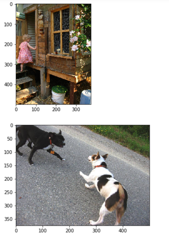

These are the first two images that you can visualize by running the following code. There are three more images that you can see after running the code block. The entire Jupyter notebook can be found here. Feel free to check out the complete code and the visualization in the provided notebook to see how the other three images look.

Pre-processing the data:

Now that we have a brief idea of how our visualization looks and the type of images we are dealing with, it is time to pre-process the captions. Let us create a function to load the appropriate files and then view them accordingly.

# Defining the function to load the captions

def load(filename):
    file = open(filename, 'r')
    text = file.read()
    file.close()
    return text

file = "captions.txt"
info = load(file)
print(info[:484])

Output:

image,caption
1000268201_693b08cb0e.jpg,A child in a pink dress is climbing up a set of stairs in an entry way .

You will receive five more outputs, but they are irrelevant to our current objective. We can see that each image is separated by a comma from its particular statement. Our goal is to separate these two entities. But firstly, let us remove the first line, which is unnecessary, and also ensure that there is no blank line at the end of the text document. Rename and save this file as captions1.txt. This step is done to ensure that, in case we make a mistake, we can redo the steps with the initial captions.txt. It is also generally good practice to save copies of your pre-processed data. Let us now visualize how your data should look.

# Delete the first line as well as the last empty line and then rename the file as captions1.txt

file = "captions1.txt"
info = load(file)
print(info[:470])

Output:

1000268201_693b08cb0e.jpg,A child in a pink dress is climbing up a set of stairs in an entry way .

In our next step, we will create a dictionary to store the image files and their respective captions accordingly. We know that each image has an option of five different captions to choose from. Hence, we will define the .jpg image as the key with their five respective captions representing the values. We will split the values appropriately and store them in a dictionary. The following function can be written as follows. Note that we are storing all this information in the data variable.

# Creating a function to create a dictionary for the images and their respective captions

def load_captions(info):
    dict_1 = dict()
    count = 0
    for line in info.split('\n'):
        
        splitter = line.split('.jpg,')
#         print(splitter)
        # The image_code and image_captions are the list of the images with their respective captions
        image_code, image_caption = splitter[0], splitter[1]
        
        # Create dictionary
        if image_code not in dict_1:
            dict_1[image_code] = list()
            
        dict_1[image_code].append(image_caption)
        
    return dict_1

data = load_captions(info)
print(len(data))

You can view the keys and values of the dictionary with the following lines.

list(data.keys())[:5]

['1000268201_693b08cb0e',
 '1001773457_577c3a7d70',
 '1002674143_1b742ab4b8',
 '1003163366_44323f5815',
 '1007129816_e794419615']

data['1000268201_693b08cb0e']

['A child in a pink dress is climbing up a set of stairs in an entry way .',
 'A girl going into a wooden building .',
 'A little girl climbing into a wooden playhouse .',
 'A little girl climbing the stairs to her playhouse .',
 'A little girl in a pink dress going into a wooden cabin .']

Our next step is to proceed with further pre-processing of the dataset and prepare the captions data by making some necessary changes. We will make sure that all the words in each of the sentences are converted to a lower case because we don't want the same word to be stored as two separate vectors during the computation of the problem. We will also remove words with a length of less than two to make sure that we remove irrelevant characters such as single letters and punctuations. The function and the code for completing this task is written as follows:

# Cleanse and pre-process the data

def cleanse_data(data):
    dict_2 = dict()
    for key, value in data.items():
        for i in range(len(value)):
            lines = ""
            line1 = value[i]
            for j in line1.split():
                if len(j) < 2:
                    continue
                j = j.lower()
                lines += j + " "
            if key not in dict_2:
                dict_2[key] = list()
            
            dict_2[key].append(lines)
            
    return dict_2

data2 = cleanse_data(data)
print(len(data2))    

Note that we are storing all this essential cleansed information in the data2 variable, which will be used throughout the rest of the programming section when required.

Update the vocabulary and data:

Once we have completed the cleansing and pre-process of the image captions in the text file, we can proceed to create a vocabulary of the words and calculate the total number of unique entities present. We will update the unique words that will be used for the computation and making predictions later on after we finish building the model architecture. Let us look at the code block that performs the following task.

# convert the following into a vocabulary of words and calculate the total words

def vocabulary(data2):
    all_desc = set()
    for key in data2.keys():
        [all_desc.update(d.split()) for d in data2[key]]
    return all_desc

# summarize vocabulary
vocabulary_data = vocabulary(data2)
print(len(vocabulary_data))

Finally, after the completion of all these essential steps, we can now update our captions1.txt file as well with the following code.

# save descriptions to file, one per line

def save_dict(data2, filename):
    lines = list()
    for key, value in data2.items():
        for desc in value:
            lines.append(key + ' ' + desc)
    data = '\n'.join(lines)
    file = open(filename, 'w')
    file.write(data)
    file.close()

save_dict(data2, 'captions1.txt')

Your text file and the data stored should look something similar to the following lines shown below.

1000268201_693b08cb0e child in pink dress is climbing up set of stairs in an entry way 
1000268201_693b08cb0e girl going into wooden building 

With the completion of the initial pre-processing of the text data, let us proceed to the next steps and construct our model architecture for predicting the appropriate captions for the respective images.

Pre-processing the Images:

Now that we are done with the pre-processing of the textual descriptions, let us proceed to pre-process the images accordingly as well. We will make use of the pre-processing function and load the image paths of each image to perform this action appropriately. Let us first look at the code and then understand our next steps. Also, note that for the rest of the article, we will make use of the following two references for simplifying the full operation image captioning task. We will use the official TensorFlow documentation on Image Captioning with Visual Attention and the following GitHub reference link for the successful computation of the following task. Let us now proceed to look at the code block that will pre-process our images accordingly.

images = 'Images/'
img = glob(images + '*.jpg')
print(len(img))

def preprocess(image_path):
    # Convert all the images to size 299x299 as expected by the inception v3 model
    img = keras.preprocessing.image.load_img(image_path, target_size=(299, 299))
    # Convert PIL image to numpy array of 3-dimensions
    x = keras.preprocessing.image.img_to_array(img)
    # Add one more dimension
    x = np.expand_dims(x, axis=0)
    # pre-process the images using preprocess_input() from inception module
    x = keras.applications.inception_v3.preprocess_input(x)
    return x

This step is one of the most critical steps as we will utilize the Inception V3 transfer learning model to convert each of the respective images into their fixed vector size. This automatic feature extraction process involves the exclusion of the final SoftMax activation function to a bottleneck of 2096 vector features. The model makes use of the pre-trained weights on the image net to achieve the computation of the following task with relative ease. The Inception V3 model is generally known to perform better on datasets with images. However, I would also recommend trying out other transfer learning models and see how they perform on the same problem.

# Load the inception v3 model
input1 = InceptionV3(weights='imagenet')

# Create a new model, by removing the last layer (output layer) from the inception v3
model = Model(input1.input, input1.layers[-2].output)

model.summary()

Once we finish the computation of pre-processing of the images, we will save all these values in a pickle file. Saving these files as individual elements will help us to utilize these models separately during the prediction process. This process can be completed with the following code block.

# Function to encode a given image into a vector of size (2048, )
def encode(image):
    image = preprocess(image) # preprocess the image
    fea_vec = model.predict(image) # Get the encoding vector for the image
    fea_vec = np.reshape(fea_vec, fea_vec.shape[1]) # reshape from (1, 2048) to (2048, )
    return fea_vec
    
 encoding = {}

for i in tqdm(img):
    encoding[i[len(images):]] = encode(i)
    
import pickle

# Save the features in the images1 pickle file
with open("images1.pkl", "wb") as encoded_pickle:
    pickle.dump(encoding, encoded_pickle)

Creating Our Data Loader:

Before we create our data loader and data generator, let us save all the essential files containing the information of the unique words to index, as well as all the indices linked to their respective words. Performing this operation is crucial for both the generator and the prediction stage of the model. We will also define a fixed maximum length for this operation so that it does not exceed the limits we set. The entire process including the saving of these necessary documents in pickle files can be done as follows:

# Create a list of all the training captions

all_train_captions = []

for key, val in data2.items():
    for cap in val:
        all_train_captions.append(cap)
        
len(all_train_captions)

# Consider only words which occur at least 10 times in the corpus

word_count_threshold = 10
word_counts = {}
nsents = 0

for sent in all_train_captions:
    nsents += 1
    for w in sent.split(' '):
        word_counts[w] = word_counts.get(w, 0) + 1

vocab = [w for w in word_counts if word_counts[w] >= word_count_threshold]
print('preprocessed words %d -> %d' % (len(word_counts), len(vocab)))

# Converting the words to indices and vice versa.

ixtoword = {}
wordtoix = {}

ix = 1
for w in vocab:
    wordtoix[w] = ix
    ixtoword[ix] = w
    ix += 1
    
vocab_size = len(ixtoword) + 1 # one for appended 0's
vocab_size

# Save the words to index and index to word as pickle files

with open("words.pkl", "wb") as encoded_pickle:
    pickle.dump(wordtoix, encoded_pickle)
    
with open("words1.pkl", "wb") as encoded_pickle:
    pickle.dump(ixtoword, encoded_pickle)
    
# convert a dictionary of clean descriptions to a list of descriptions

def to_lines(descriptions):
    all_desc = list()
    for key in descriptions.keys():
        [all_desc.append(d) for d in descriptions[key]]
    return all_desc

# calculate the length of the description with the most words
def max_length(descriptions):
    lines = to_lines(descriptions)
    return max(len(d.split()) for d in lines)

# determine the maximum sequence length
max_length = max_length(data2)
print('Description Length: %d' % max_length)

Build the Generator:

Our final step is to create the data generator, which will load the entire information of the image vectors, the respective descriptions of the model, the maximum length, the fixed words to index values, the number of steps to run per epoch, and all other elementary actions. Each image is converted into its respective feature length, and all the descriptions are padded accordingly such that when passed through an LSTM type structure, we can make predictions of future words. The TensorFlow documentation approach with the Sequence to Sequence with Attention modeling is better to obtain higher accuracies and better training with the tf.data() method. However, we will use a slightly simpler approach for this problem to achieve quicker results.

# data generator, intended to be used in a call to model.fit_generator()

def data_generator(descriptions, photos, wordtoix, max_length, num_photos_per_batch):
    X1, X2, y = list(), list(), list()
    n=0
    # loop for ever over images
    while 1:
        for key, desc_list in descriptions.items():
            n+=1
            # retrieve the photo feature
            photo = photos[key+'.jpg']
            for desc in desc_list:
                # encode the sequence
                seq = [wordtoix[word] for word in desc.split(' ') if word in wordtoix]
                # split one sequence into multiple X, y pairs
                for i in range(1, len(seq)):
                    # split into input and output pair
                    in_seq, out_seq = seq[:i], seq[i]
                    # pad input sequence
                    in_seq = pad_sequences([in_seq], maxlen=max_length)[0]
                    # encode output sequence
                    out_seq = to_categorical([out_seq], num_classes=vocab_size)[0]
                    # store
                    X1.append(photo)
                    X2.append(in_seq)
                    y.append(out_seq)
            # yield the batch data
            if n==num_photos_per_batch:
                yield ([array(X1), array(X2)], array(y))
                X1, X2, y = list(), list(), list()
                n=0

With the construction of the training generator to load our values appropriately, we can proceed to the final step of building the model architecture to accomplish the task of image captioning.

Building The Final Model Architecture:

Now that we have completed most of the individual steps for pre-processing both the caption labels, the textual descriptions, and the image data, we can finally proceed towards the construction of the model. Before we construct our model, however, we need to create word embedding vectors for each unique word for a fixed length. The word embedding method is used to map every single index of words to a 200 length vector to make it an uniformly sized distribution. Please download the following glove vector from this link. The pre-trained glove.6B.200d.txt is used for this model to create an embedding matrix of an uniformly distributed 200 length for all the unique words. The following code block performs the required operations.

# Download, install, and then Load the Glove vectors
# https://github.com/stanfordnlp/GloVe

embeddings_index = {} # empty dictionary
f = open('glove.6B.200d.txt', encoding="utf-8")

for line in f:
    values = line.split()
    word = values[0]
    coefs = np.asarray(values[1:], dtype='float32')
    embeddings_index[word] = coefs
f.close()
print('Found %s word vectors.' % len(embeddings_index))

embedding_dim = 200

# Get 200-dim dense vector for each of the 10000 words in out vocabulary
embedding_matrix = np.zeros((vocab_size, embedding_dim))

for word, i in wordtoix.items():
    #if i < max_words:
    embedding_vector = embeddings_index.get(word)
    if embedding_vector is not None:
        # Words not found in the embedding index will be all zeros,
        embedding_matrix[i] = embedding_vector
        
embedding_matrix.shape

Output:

Found 400001 word vectors.
(1976, 200)

Finally, let us define the LSTM and embedding layers to create our model architecture. For this model, we will make use of two inputs, namely the image vectors and the word embeddings of the captions, for making the predictions. The embedding vector is passed through an LSTM architecture which will learn how to make the appropriate word predictions. The image vector and the LSTM predictions are combined together as one unit and passed through some dense layers and a SoftMax activation function, which is equivalent to the size of the pre-defined vocabulary. Finally, we will construct this model and begin with our training process.

from tensorflow.keras.layers import Dense, Input, Conv2D, MaxPool2D, LSTM, add
from tensorflow.keras.layers import Activation, Dropout, Flatten, Embedding
from tensorflow.keras.models import Model

inputs1 = Input(shape=(2048,))
fe1 = Dropout(0.5)(inputs1)
fe2 = Dense(256, activation='relu')(fe1)

inputs2 = Input(shape=(max_length,))
se1 = Embedding(vocab_size, embedding_dim, mask_zero=True)(inputs2)
se2 = Dropout(0.5)(se1)
se3 = LSTM(256)(se2)

decoder1 = add([fe2, se3])
decoder2 = Dense(256, activation='relu')(decoder1)
outputs = Dense(vocab_size, activation='softmax')(decoder2)

model = Model(inputs=[inputs1, inputs2], outputs=outputs)
model.summary()

Model: "model_1"
__________________________________________________________________________________________________
Layer (type)                    Output Shape         Param #     Connected to                     
==================================================================================================
input_3 (InputLayer)            [(None, 33)]         0                                            
__________________________________________________________________________________________________
input_2 (InputLayer)            [(None, 2048)]       0                                            
__________________________________________________________________________________________________
embedding (Embedding)           (None, 33, 200)      395200      input_3[0][0]                    
__________________________________________________________________________________________________
dropout (Dropout)               (None, 2048)         0           input_2[0][0]                    
__________________________________________________________________________________________________
dropout_1 (Dropout)             (None, 33, 200)      0           embedding[0][0]                  
__________________________________________________________________________________________________
dense (Dense)                   (None, 256)          524544      dropout[0][0]                    
__________________________________________________________________________________________________
lstm (LSTM)                     (None, 256)          467968      dropout_1[0][0]                  
__________________________________________________________________________________________________
add (Add)                       (None, 256)          0           dense[0][0]                      
                                                                 lstm[0][0]                       
__________________________________________________________________________________________________
dense_1 (Dense)                 (None, 256)          65792       add[0][0]                        
__________________________________________________________________________________________________
dense_2 (Dense)                 (None, 1976)         507832      dense_1[0][0]                    
==================================================================================================
Total params: 1,961,336
Trainable params: 1,961,336
Non-trainable params: 0
__________________________________________________________________________________________________

Now that we have finished the construction of our overall model architecture, let us proceed to compile the model with the categorical cross-entropy loss function and the Adam optimizer. I will train the model for about ten epochs due to time constraints. However, you can choose to explore and train them for a higher number of epochs at your convenience.

model.layers[2].set_weights([embedding_matrix])
model.layers[2].trainable = False

model.compile(loss='categorical_crossentropy', optimizer='adam')

epochs = 10
number_pics_per_bath = 3
steps = len(data2)//number_pics_per_bath

features = pickle.load(open("images1.pkl", "rb"))

# https://stackoverflow.com/questions/58352326/running-the-tensorflow-2-0-code-gives-valueerror-tf-function-decorated-functio

tf.config.run_functions_eagerly(True)

for i in range(epochs):
    generator = data_generator(data2, features, wordtoix, max_length, number_pics_per_bath)
    model.fit(generator, epochs=1, steps_per_epoch=steps, verbose=1)
    model.save('model_' + str(i) + '.h5')

Output:

2697/2697 [==============================] - 986s 365ms/step - loss: 4.5665
2697/2697 [==============================] - 983s 365ms/step - loss: 3.4063
2697/2697 [==============================] - 987s 366ms/step - loss: 3.1929
2697/2697 [==============================] - 987s 366ms/step - loss: 3.0570
2697/2697 [==============================] - 989s 366ms/step - loss: 2.9662
2697/2697 [==============================] - 995s 369ms/step - loss: 2.9011
2697/2697 [==============================] - 989s 367ms/step - loss: 2.8475
2697/2697 [==============================] - 986s 366ms/step - loss: 2.8062
2697/2697 [==============================] - 986s 366ms/step - loss: 2.7689
2697/2697 [==============================] - 987s 365ms/step - loss: 2.7409

We can notice that with just ten epochs of training, our loss has significantly reduced from its initial values. I have trained the model for only ten epochs because you can notice that each epoch takes approximately 1000 seconds to run on my GPU. If you have a faster computing GPU or more time, you can train the model for a higher number of epochs to achieve an overall better result.

Making Predictions:

While making the appropriate predictions, we will make use of a separate notebook. Doing so is a demonstration that all the saved files and models can be used independently for making the most precise predictions on the given image data. Let us firstly import all the essential libraries and start the particular task.

Importing the required libraries

These are some of the essential libraries you must import for defining the prediction function.

import tensorflow as tf
from tensorflow import keras
from tensorflow.keras.models import load_model
from tensorflow.keras.preprocessing.sequence import pad_sequences
import numpy as np
import matplotlib.pyplot as plt
import pickle

Loading the respective features:

Let us load all the saved files into their respective variables. This process is done as follows.

features = pickle.load(open("images1.pkl", "rb"))
model = load_model('model_9.h5')
images = "Images/"
max_length = 33
words_to_index = pickle.load(open("words.pkl", "rb"))
index_to_words = pickle.load(open("words1.pkl", "rb"))

Making the predictions:

Finally, let us define the respective function that will take in the images, load their vectors, create word embedding, and utilize the saved model for making the appropriate predictions. Let us randomly test on two images and visualize their respective outcomes.

def Image_Caption(picture):
    in_text = 'startseq'
    for i in range(max_length):
        sequence = [words_to_index[w] for w in in_text.split() if w in words_to_index]
        sequence = pad_sequences([sequence], maxlen=max_length)
        yhat = model.predict([picture,sequence], verbose=0)
        yhat = np.argmax(yhat)
        word = index_to_words[yhat]
        in_text += ' ' + word
        if word == 'endseq':
            break
    final = in_text.split()
    final = final[1:-1]
    final = ' '.join(final)
    return final

I will randomly select an image, and we will try to visualize the outputs produced by our model for a couple of images.

z = 20
pic = list(features.keys())[z]
image = features[pic].reshape((1,2048))
x = plt.imread(images+pic)
plt.imshow(x)
plt.show()
print("Caption:", Image_Caption(image))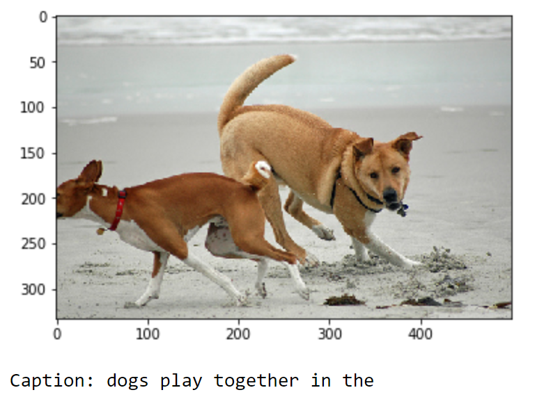

z = 100
pic = list(features.keys())[z]
image = features[pic].reshape((1,2048))
x = plt.imread(images+pic)
plt.imshow(x)
plt.show()
print("Caption:", Image_Caption(image))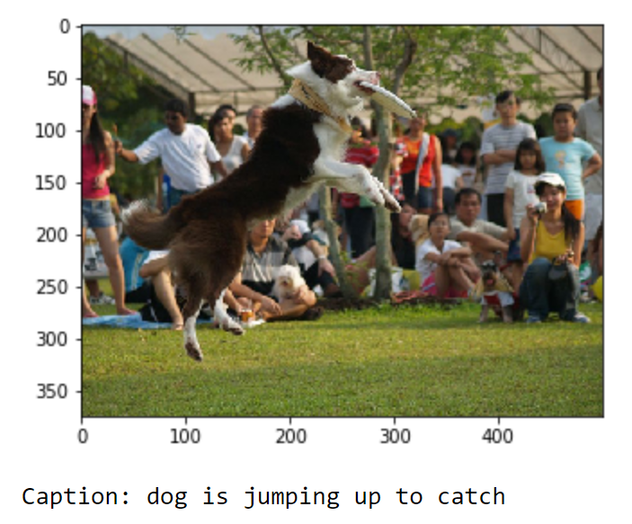

We can notice that the performance of our image captioning model is quite good for just ten epochs of training and a small dataset. While the image captioning task works fairly decent, it is worth noting that the loss can further be reduced to achieve higher accuracy and precision. The two main changes and improvements that can be made are increasing the size of the dataset and running the following computation on the current model for more epochs. A Sequence to Sequence with Attention model can also be used for achieving better results. Other experiments on different types of transfer learning models can be conducted as well.

Conclusion:

In this demonstration of image caption generation with Keras and TensorFlow, we showed how to use previously identified text caption data from the Flickr dataset in order to produce novel captions. Included in this process were the steps for loading up the relevant libraries, pre-processing of the image and text data, creating the data loader and generator, and finally the construction of an LSTM architecture to generate the predicted captions. Users can follow along in further detail and attempt to recreate this work by using the public notebook on Gradient-AI's GitHub.