A Complete Intuitive Guide To Transfer Learning (Part 1)

Advancements in deep learning have been rapid over the past decade. While the discovery of neural networks happened almost six decades ago with the invention of the first artificial neural network in 1958 by psychologist Frank Rosenblatt (called the "perceptron"), the developments in the field did not gain true popularity until about a decade ago. The most popular achievement in 2009 was the creation of ImageNet. ImageNet is a humungous visual dataset that has led to some of the best modern-day deep learning and computer vision projects.

ImageNet consists of over 14 million images that are hand-annotated to indicate the representation of particular objects in each picture. Over 1 million images include specific bounding boxes as well. These bounding boxes are useful for several computer vision applications such as object detection, object tracking, and much more. We will learn more about the significance of ImageNet as we proceed further in this 2-part series.

This article (Part 1) will cover a complete theoretical guide to gaining a deep intuition on transfer learning. In the next part of this series, we will dive deeper into a practical, hands-on guide, and implement some transfer learning models including a face recognition project. Let's quickly take a look at the table of contents to understand the concepts that will be covered in this article. Feel free to skip ahead to the concepts that you want to explore the most. However, if you are new to the topic, it is advisable to go through the entire article.

Table of Contents

• Introduction
• Understanding convolutional neural networks
  1. How a CNN works
  2. Basic implementation of CNNs
  3. Diving into the max-pooling layer
• Learning transfer learning
• Intuition behind fine-tuning
  1. Understanding fine-tuning
  2. Best practices
• Exploring several transfer learning models
  1. AlexNet
  2. VGG-16
• Conclusion

Introduction

With all the accomplishments and continuous progression that we have made in the field of deep learning, it would be a shame if we did not take advantage of all this learned knowledge to help perform complicated tasks. One such common practice is the use of transfer learning, where models with pre-trained weights are applied in new contexts.

In this article, we will focus in particular on convolutional neural networks (CNNs), which are utilized in most computer vision tasks. After we gain a basic intuition of CNNs, we will proceed to learn more about transfer learning and several crucial aspects related to this topic, including fine-tuning. We will finally explore a few typical transfer learning models and their use cases. In the next article, we will dive into the practical aspects of their implementation in the context of a face recognition problem.

Understanding Convolutional Neural Networks

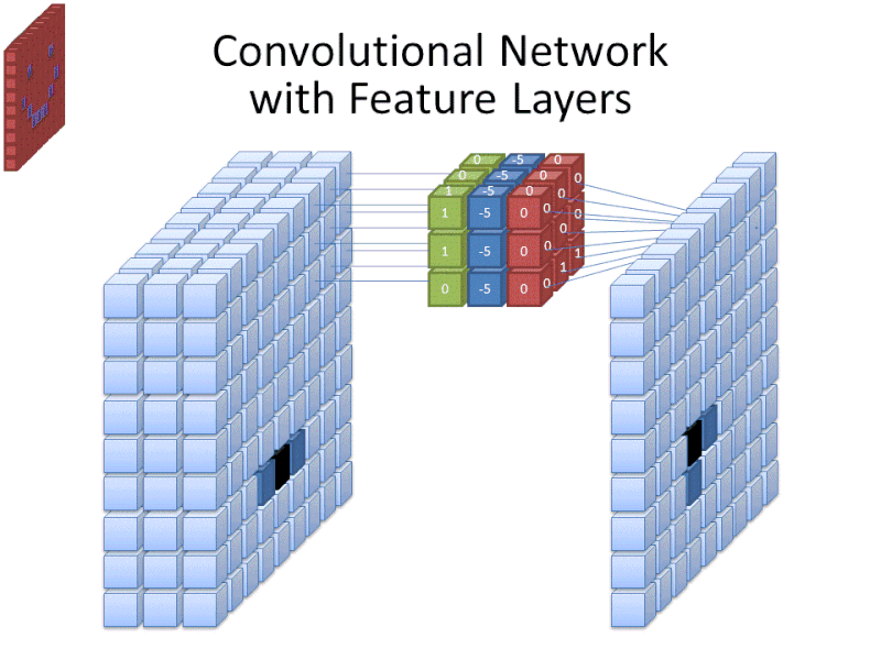
Convolutional neural networks are a class of artificial deep neural networks. They are also referred to as ConvNets, or CNNs for short. Convolutional neural networks are loosely inspired by certain biological processes, mainly from the activity of neurons in the animal visual cortex. To gain an overall understanding of their working procedure in simple terms, it must be noted that these CNNs utilize filters to turn complex patterns into something smaller and simpler to analyze, interpret, and easily visualize. We'll go into more detail about this in Part 2.

Mostly the 2-dimensional convolutional neural networks are used for solving computer vision problems with deep learning. These include tasks related to handwriting recognition, gesture recognition, emotion recognition, and much more. Although their main use is for computer vision applications, they are not limited to them. With the use of 1-dimensional convolutional layers, we can even achieve decent accuracy for predictions in natural language processing tasks. However, we will limit ourselves to the study of 2-D convolutional layers for the purposes of this article.

In the upcoming sections, we will go through a detailed analysis of the complete working of Convolutional Neural Networks, understand their basic implementation, and finally, cover the max-pooling layer. Without further ado, let's get started.

How a CNN works

In the above image, we have a $(6\times 6)$ matrix that is convolved with a kernel of size $(3 \times 3)$. Convolutional layers involve the use of a kernel that is "convolved" over the layer input to produce a tensor of outputs. The $(3 \times 3)$ kernel in the above image is usually referred to as the "Sobel Edge Detector", or "Horizontal Edge Detector". Usually, when a $(6\times 6)$ matrix is convolved with a $(3\times 3)$ kernel, the resulting output matrix will have a shape of $(4\times 4)$. To reach this result, a series of component-wise multiplications are performed. Convolution, in other words, is basically a method of finding the suitable dot product.

As shown in the image above, we end up with a $(6\times 6)$ matrix which looks like the following:

array([[9, 8, 6, 6, 8, 9],
       [8, 2, 1, 1, 2, 8],
       [6, 1, 0, 0, 1, 6],
       [6, 1, 0, 0, 1, 6],
       [8, 2, 1, 1, 2, 8],
       [9, 8, 6, 6, 8, 9]])

The reason our output matrix is the same size as our input matrix is due to the implementation of padding. With padding, the initial $(6\times 6)$ input matrix is "padded" with an additional layer around the entire matrix, and hence, it is converted into an $(8\times 8)$ matrix. There are two main types of padding operations:

1. Zero Padding: Adding a layer of zeros around the entire matrix. This method is usually the more common approach.
2. Same value padding: Trying to replicate the values in the nearest rows or columns.

The other essential concept to know when working with CNNs is that of strides. Strides are the number of shifts that are taken into consideration for each particular evaluation. We can notice that there is only a single stride in the above picture. We can have any number of strides and padding values in a particular implementation of a convolutional layer. The number of filters, the kernel size, the type of padding, the number of strides, and the activation function (among other parameters) can be implemented with TensorFlow and Keras. The final output size is determined by the input shape, the kernel size, the type of padding, and the number of strides.

Basic implementation of CNNs

After understanding the complete working procedure of convolutional layers and convolutional neural networks in general, let us now look at implementing some of these architectures with the TensorFlow and Keras deep learning frameworks. Before you dive into the code, it is highly recommended that you check out my previous articles on these topics that cover both TensorFlow and Keras in detail. Let us explore a simple sample code block covering how a convolutional layer and a max-pooling layer are implemented.

from tensorflow.keras.layers import Convolution2D, MaxPooling2D

Convolution2D(512, kernel_size=(3,3), activation='relu', padding="same")
MaxPooling2D((2,2), strides=(2,2))

An alternate way of implementing the exact same code is written as follows:

from tensorflow.keras.layers import Conv2D, MaxPool2D

Conv2D(512, kernel_size=(3,3), activation='relu', padding="same")
MaxPool2D((2,2), strides=(2,2))

Note that these functions are aliases of each other. They perform the exact same functionality, and you can use either alternative according to your convenience. I would recommend testing out these methods yourself. It is worth noting that some of the aliases might be deprecated in future Keras versions. It is always a good habit to stay up to date with the developments of these libraries.

keras.layers.Conv2D
keras.layers.Convolution2D
keras.layers.convolutional.Conv2D
keras.layers.convolutional.Convolution2D

Each line above holds the same meaning and is an alias of one another. You can effectively use any of these methods at your convenience.

Diving into the max-pooling layer

The max-pooling layer is used to downsample the spatial dimensions of the convolutional layers. This process is mainly done to create location invariance while operating on images. In a max-pooling layer, particular sets of matrices are chosen with respect to the kernel size and the strides mentioned. Once these matrices are chosen, the largest value is chosen as the output of that particular cell. The operation is repeated across other smaller matrices to receive the required outputs for each cell. The above image depicts an example of RoI pooling of size $(2 \times 2)$. In this example the region proposal (an input parameter) has a size of $(7 \times 5)$.

Most convolutional layers are followed by a max-pooling layer. Max-pooling is crucial for the optimal performance of convolutional neural networks. These layers introduce location invariance, which means the location of features in an image will not affect the network's ability to detect them. They also introduce other types of invariances, such as scale invariance (where the size or shape of an image does not affect the outcome) and rotation invariance (where the rotation angle of the image does not affect the outcome), among many other significant advantages.

Learning Transfer Learning

Nowadays, only rarely will you witness the implementation of a complete neural network with random weight initializations built from scratch. Typical datasets are much too small to achieve high-performing models when trained only on this task-specific data. The most common practice in deep learning today is to instead do transfer learning.

Transfer learning involves using a network that has already been trained on a large corpus of data, then re-training it (or "fine-tuning" it) on a smaller dataset specific to the task at hand. These models are typically trained on large datasets like ImageNet, which include millions of images. The weights learned from this pre-training are saved and used for model initialization.

There are three main scenarios for transfer learning: ConvNets as fixed feature extractors, fine-tuning, and pre-trained models. In this section of the article, we will focus on ConvNets as a fixed feature extractor and pre-trained models. In the upcoming section, we will go into further depth on the topic of fine-tuning.

When using a ConvNet as a fixed feature extractor, the typical operation is to replace the final output layer with one that will contain the required number of output nodes for the multi-class computation with the help of the SoftMax function. On the other hand, pre-trained models are models with the best weights stored as a checkpoint, and can be utilized for the direct testing of performance on datasets without including any additional training procedure. The main use case for this scenario is when a network will take a long time to train (even with powerful GPUs), you can instead use the best saved weights to obtain suitable results on the test data. An example of the following is the Caffe Model Zoo, where people share their network weights so others can use them for their own projects.

Intuition behind fine-tuning

One of the most important strategies in modern deep learning is fine-tuning. In the upcoming sections, our primary objective will be to understand the concept of fine-tuning and the best practices that will lead the programmer to obtain optimal results.

Understanding fine-tuning

Fine-tuning involves not only replacing the final dense output layer from the pre-trained network we're using, but also a retraining of the classifier on the new dataset. The most common tactic among practitioners is to fine-tune only the top layer of the transfer learning architectures to avoid over-fitting. Hence, in most scenarios, the earlier layers are usually kept as-is.

Best practices

There are several factors that must be considered in practice before fine-tuning your network: whether the new dataset is smaller or larger than the one the network was originally trained on, and how similar it is to that original dataset.

1. The new dataset is small and similar to the original dataset - For smaller datasets with a strong resemblance to the original dataset, it is preferable to skip the method of fine-tuning because it could potentially lead to over-fitting.
2. The new dataset is large and similar to the original dataset - This scenario is perfect for transfer learning. When we have a large dataset with a strong resemblance to the original dataset, we can fine-tune accordingly to achieve fabulous results.
3. The new dataset is small but very different from the original dataset - Similar to our previous discussion, since the dataset is quite small, the best idea would be to use a linear classifier. However, since the new dataset is very different from the original dataset, it would potentially be better to train a SVM classifier from activations somewhere earlier in the network for better performance.
4. The new dataset is large and very different from the original dataset - When the dataset is large, fine-tuning is never a bad idea. Even though the new dataset is quite different from the original one, we can often get away with excluding only the top portion of the network.

I like to use the following code for transfer learning models being fine-tuned.

# Convolutional Layer
Conv1 = Conv2D(filters=32, kernel_size=(3,3), strides=(1,1), padding='valid',
               data_format='channels_last', activation='relu', 
               kernel_initializer=keras.initializers.he_normal(seed=0), 
               name='Conv1')(input_layer)

# MaxPool Layer
Pool1 = MaxPool2D(pool_size=(2,2),strides=(2,2),padding='valid', 
                  data_format='channels_last',name='Pool1')(Conv1)

# Flatten
flatten = Flatten(data_format='channels_last',name='Flatten')(Pool1)

# Fully Connected layer-1
FC1 = Dense(units=30, activation='relu', 
            kernel_initializer=keras.initializers.glorot_normal(seed=32), 
            name='FC1')(flatten)

# Fully Connected layer-2
FC2 = Dense(units=30, activation='relu', 
            kernel_initializer=keras.initializers.glorot_normal(seed=33),
            name='FC2')(FC1)

# Output layer
Out = Dense(units=num_classes, activation='softmax', 
            kernel_initializer=keras.initializers.glorot_normal(seed=3), 
            name='Output')(FC2)

Regardless of what you choose to work with, it is essential to note that experimentation and numerous implementations are required to ensure the best results are obtained. The beauty of deep learning is the factor of randomness. Many of the best results are obtained only by trying out lots of new methods.

Now that we have a decent understanding of the working of convolutional neural networks and transfer learning, let's explore a few transfer learning models based on their significance in history and those which are commonly used to achieve quick, high-quality results. For further reading on the topic of fine-tuning, I would highly recommend checking out Stanford's website for transfer learning from the Convolutional Neural Networks for Visual Recognition course from the following website.

Exploring several transfer learning models

In this section of the article, we will look into a couple of transfer learning architectures, namely AlexNet and VGG-16. Let us explore these models briefly with some image representations to get an overview of these topics. In the next article on "The Complete Practical Guide To Transfer Learning", we will explore three more different types of transfer learning models with some practical implementations, namely ResNet50, InceptionV3, and MobileNetV2. For now, let us view and understand the AlexNet and VGG-16 architectures.

1. AlexNet

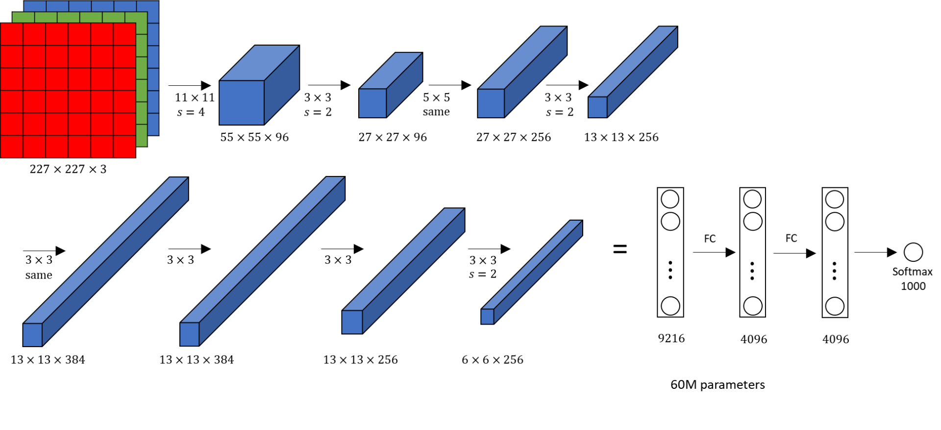
After the initial success of  LeNet-5, AlexNet followed with an increase in depth. This architecture was proposed in 2012 in the research paper titled "ImageNet Classification with Deep Convolution Neural Network" by Alex Krizhevsky and his colleagues. AlexNet won the ImageNet large-scale visual recognition challenge in the same year. In the AlexNet architecture, we have an input image that is passed through a convolutional layer and max-pooling layer twice. Then, we pass it through a series of three convolutional layers followed by a single max-pooling layer. After this step, we have three hidden layers followed by the output. In AlexNet, the overall computation in the final stage would result in a 4096-D vector for every image that contains the activations of the hidden layer immediately before the classifier. While most of the layers would utilize the ReLU activation function, the final layer makes use of the SoftMax activation.

2. VGG-16

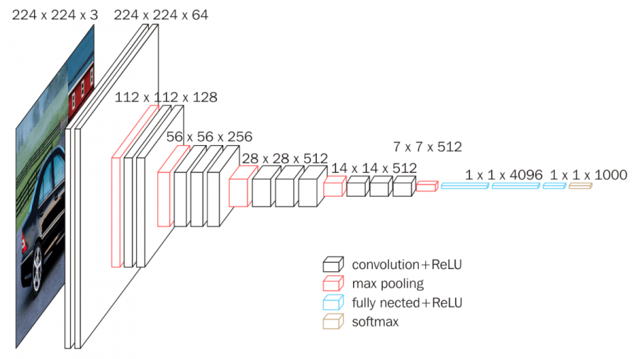
The "VGG" in VGG-16 stands for "Visual Geometric Group". It is associated with the Department of Science and Engineering at Oxford University. In the initial stages, this architecture was used to study the accuracies of large-scale classification. Now, the most common use for the VGG-16 architecture is mainly for solving tasks such as face recognition and image classification. From the above image representation, we can notice that an RGB image of size $(224, 224)$ is usually passed through its layers. A $2X$ convolutional layer followed by a max-pooling layer is utilized three times, and then a $3X$ convolutional layer followed by a max-pooling layer is utilized two times. Finally, three hidden layers are followed by an output layer with 1000 nodes achieved by a SoftMax activation function. All the other layers usually utilize the ReLU activation function.

Conclusion

With our new knowledge of transfer learning models, we have understood some of the common tools used to solve complicated tasks in deep learning quicker. Deep learning has a long and steep learning curve with tons of discoveries to be made. Transfer learning has enabled researchers in the field to achieve better results with less data.

In this article, we covered most of the essential concepts required for the understanding of how transfer learning works and how these models are used in practice. We started by taking a look at convolutional neural networks (CNNs), one of the most commonly used models for transfer learning. We then understood the numerous methods of the implementation of transfer learning models and focused on the fine-tuning aspect of their implementation. Finally, we explored a few of the many transfer learning models that are available to us to create unique projects.

While the focus of this article has been on the theoretical aspects of transfer learning, we are only just getting started! In the next article, we will dive into several popular transfer learning techniques and implement a face recognition project. We will discuss how we can construct such a model from scratch and utilize a few popular transfer learning models for a comparison of how they work on a real-time problem. Until then, keep learning and exploring!