Continuing my series on building classical convolutional neural networks that revolutionized the field of computer vision in the last 1-2 decades, we next will build VGG, a very deep convolutional neural network, from scratch using PyTorch. You can see the previous articles in the series on my profile, mainly LeNet5 and AlexNet.
As before, we will be looking into the architecture and intuition behind VGG and how the results were at that time. We will then explore our dataset, CIFAR100, and load into our program using memory-efficient code. Then, we will implement VGG16 (number refers to the number of layers, there are two versions basically VGG16 and VGG19) from scratch using PyTorch and then train it our dataset along with evaluating it on our test set to see how it performs on unseen data
VGG
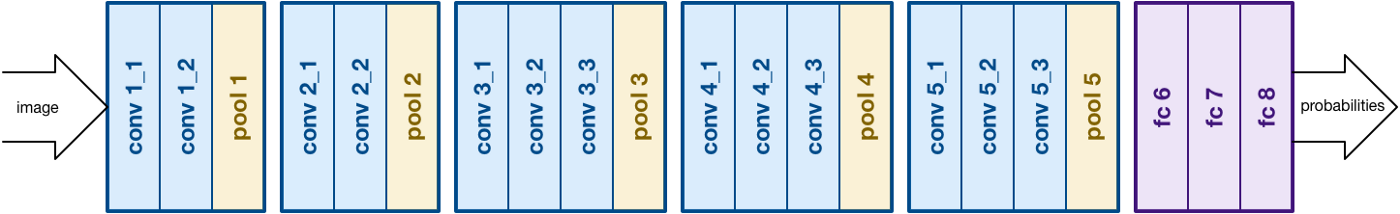
Building on the work of AlexNet, VGG focuses on another crucial aspect of Convolutional Neural Networks (CNNs), depth. It was developed by Simonyan and Zisserman. It normally consists of 16 convolutional layers but can be extended to 19 layers as well (hence the two versions, VGG-16 and VGG-19). All the convolutional layers consists of 3x3 filters. You can read more about the network in the official paper here
Data Loading
Dataset
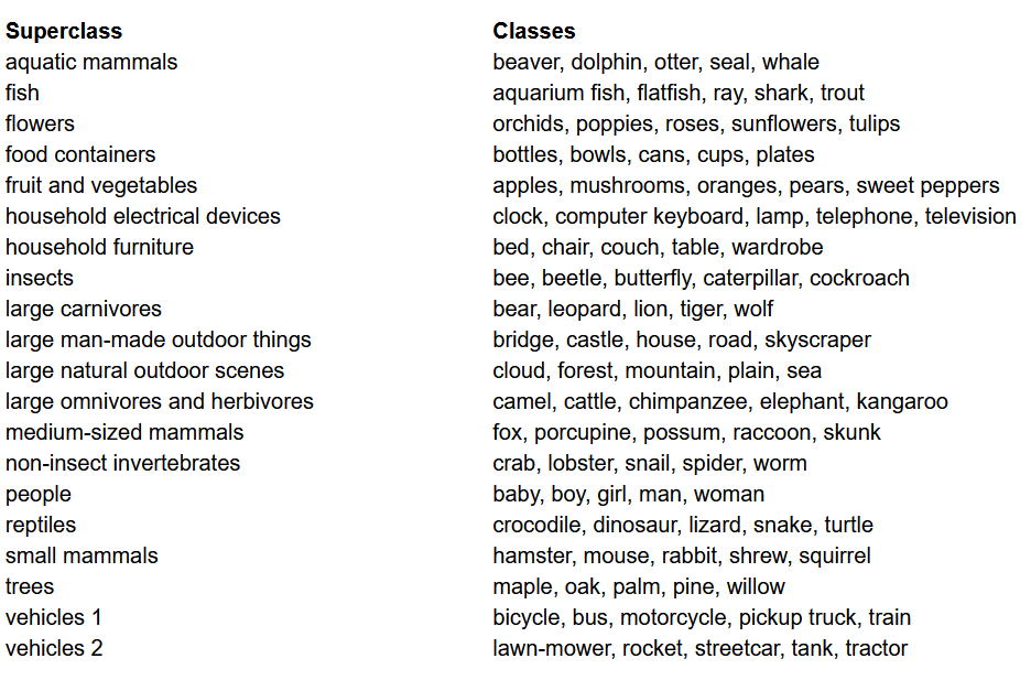
Before building the model, one of the most important things in any Machine Learning project is to load, analyze, and pre-process the dataset. In this article, we'll be using the CIFAR-100 dataset. This dataset is just like the CIFAR-10, except it has 100 classes containing 600 images each. There are 500 training images and 100 testing images per class. The 100 classes in the CIFAR-100 are grouped into 20 superclasses. Each image comes with a "fine" label (the class to which it belongs) and a "coarse" label (the superclass to which it belongs). We'll be using the "fine" label here. Here's the list of classes in the CIFAR-100:
Importing the libraries
We'll be working mainly with torch (used for building the model and training), torchvision (for data loading/processing, contains datasets and methods for processing those datasets in computer vision), and numpy (for mathematical manipulation). We will also be defining a variable device so that the program can use GPU if available
import numpy as np
import torch
import torch.nn as nn
from torchvision import datasets
from torchvision import transforms
from torch.utils.data.sampler import SubsetRandomSampler


# Device configuration
device = torch.device('cuda' if torch.cuda.is_available() else 'cpu')
Loading the Data
torchvision is a library that provides easy access to tons of computer vision datasets and methods to pre-process these datasets in an easy and intuitive manner
- We define a function
data_loaderthat returns either train/validation data or test data depending on the arguments - We start by defining the variable
normalizewith the mean and standard deviations of each of the channel (red, green, and blue) in the dataset. These can be calculated manually, but are also available online. This is used in thetransformvariable where we resize the data, convert it to tensors and then normalize it - If the
testargument is true, we simply load the test split of the dataset and return it using data loaders (explained below) - In case
testis false (default behaviour as well), we load the train split of the dataset and randomly split it into train and validation set (0.9:0.1) - Finally, we make use of data loaders. This might not affect the performance in the case of a small dataset like CIFAR100, but it can really impede the performance in case of large datasets and is generally considered a good practice. Data loaders allow us to iterate through the data in batches, and the data is loaded while iterating and not all at once in start into your RAM
def data_loader(data_dir,
                batch_size,
                random_seed=42,
                valid_size=0.1,
                shuffle=True,
                test=False):

    normalize = transforms.Normalize(
        mean=[0.4914, 0.4822, 0.4465],
        std=[0.2023, 0.1994, 0.2010],
    )

    # define transforms
    transform = transforms.Compose([
            transforms.Resize((227,227)),
            transforms.ToTensor(),
            normalize,
    ])

    if test:
        dataset = datasets.CIFAR100(
          root=data_dir, train=False,
          download=True, transform=transform,
        )

        data_loader = torch.utils.data.DataLoader(
            dataset, batch_size=batch_size, shuffle=shuffle
        )

        return data_loader

    # load the dataset
    train_dataset = datasets.CIFAR100(
        root=data_dir, train=True,
        download=True, transform=transform,
    )

    valid_dataset = datasets.CIFAR10(
        root=data_dir, train=True,
        download=True, transform=transform,
    )

    num_train = len(train_dataset)
    indices = list(range(num_train))
    split = int(np.floor(valid_size * num_train))

    if shuffle:
        np.random.seed(random_seed)
        np.random.shuffle(indices)

    train_idx, valid_idx = indices[split:], indices[:split]
    train_sampler = SubsetRandomSampler(train_idx)
    valid_sampler = SubsetRandomSampler(valid_idx)

    train_loader = torch.utils.data.DataLoader(
        train_dataset, batch_size=batch_size, sampler=train_sampler)

    valid_loader = torch.utils.data.DataLoader(
        valid_dataset, batch_size=batch_size, sampler=valid_sampler)

    return (train_loader, valid_loader)


# CIFAR100 dataset
train_loader, valid_loader = data_loader(data_dir='./data',
                                         batch_size=64)

test_loader = data_loader(data_dir='./data',
                              batch_size=64,
test=True)Bring this project to life
VGG16 from Scratch
To build the model from scratch, we need to first understand how model definitions work in torch and the different types of layers that we'll be using here:
- Every custom models need to inherit from the
nn.Moduleclass as it provides some basic functionality that helps the model to train. - Secondly, there are two main things that we need to do. First, define the different layers of our model inside the
__init__function and the sequence in which these layers will be executed on the input inside theforwardfunction
Let's now define the various types of layers that we are using here:
nn.Conv2d: These are the convolutional layers that accepts the number of input and output channels as arguments, along with kernel size for the filter. It also accepts any strides or padding if you want to apply thosenn.BatchNorm2d: This applies batch normalization to the output from the convolutional layernn.ReLU: This is the activation applied to various outputs in the networknn.MaxPool2d: This applies max pooling to the output with the kernel size givennn.Dropout: This is used to apply dropout to the output with a given probabilitynn.Linear: This is basically a fully connected layernn.Sequential: This is technically not a type of layer but it helps in combining different operations that are part of the same step
Using this knowledge, we can now build our VGG16 model using the architecture in the paper:
class VGG16(nn.Module):
    def __init__(self, num_classes=10):
        super(VGG16, self).__init__()
        self.layer1 = nn.Sequential(
            nn.Conv2d(3, 64, kernel_size=3, stride=1, padding=1),
            nn.BatchNorm2d(64),
            nn.ReLU())
        self.layer2 = nn.Sequential(
            nn.Conv2d(64, 64, kernel_size=3, stride=1, padding=1),
            nn.BatchNorm2d(64),
            nn.ReLU(),
            nn.MaxPool2d(kernel_size = 2, stride = 2))
        self.layer3 = nn.Sequential(
            nn.Conv2d(64, 128, kernel_size=3, stride=1, padding=1),
            nn.BatchNorm2d(128),
            nn.ReLU())
        self.layer4 = nn.Sequential(
            nn.Conv2d(128, 128, kernel_size=3, stride=1, padding=1),
            nn.BatchNorm2d(128),
            nn.ReLU(),
            nn.MaxPool2d(kernel_size = 2, stride = 2))
        self.layer5 = nn.Sequential(
            nn.Conv2d(128, 256, kernel_size=3, stride=1, padding=1),
            nn.BatchNorm2d(256),
            nn.ReLU())
        self.layer6 = nn.Sequential(
            nn.Conv2d(256, 256, kernel_size=3, stride=1, padding=1),
            nn.BatchNorm2d(256),
            nn.ReLU())
        self.layer7 = nn.Sequential(
            nn.Conv2d(256, 256, kernel_size=3, stride=1, padding=1),
            nn.BatchNorm2d(256),
            nn.ReLU(),
            nn.MaxPool2d(kernel_size = 2, stride = 2))
        self.layer8 = nn.Sequential(
            nn.Conv2d(256, 512, kernel_size=3, stride=1, padding=1),
            nn.BatchNorm2d(512),
            nn.ReLU())
        self.layer9 = nn.Sequential(
            nn.Conv2d(512, 512, kernel_size=3, stride=1, padding=1),
            nn.BatchNorm2d(512),
            nn.ReLU())
        self.layer10 = nn.Sequential(
            nn.Conv2d(512, 512, kernel_size=3, stride=1, padding=1),
            nn.BatchNorm2d(512),
            nn.ReLU(),
            nn.MaxPool2d(kernel_size = 2, stride = 2))
        self.layer11 = nn.Sequential(
            nn.Conv2d(512, 512, kernel_size=3, stride=1, padding=1),
            nn.BatchNorm2d(512),
            nn.ReLU())
        self.layer12 = nn.Sequential(
            nn.Conv2d(512, 512, kernel_size=3, stride=1, padding=1),
            nn.BatchNorm2d(512),
            nn.ReLU())
        self.layer13 = nn.Sequential(
            nn.Conv2d(512, 512, kernel_size=3, stride=1, padding=1),
            nn.BatchNorm2d(512),
            nn.ReLU(),
            nn.MaxPool2d(kernel_size = 2, stride = 2))
        self.fc = nn.Sequential(
            nn.Dropout(0.5),
            nn.Linear(7*7*512, 4096),
            nn.ReLU())
        self.fc1 = nn.Sequential(
            nn.Dropout(0.5),
            nn.Linear(4096, 4096),
            nn.ReLU())
        self.fc2= nn.Sequential(
            nn.Linear(4096, num_classes))

    def forward(self, x):
        out = self.layer1(x)
        out = self.layer2(out)
        out = self.layer3(out)
        out = self.layer4(out)
        out = self.layer5(out)
        out = self.layer6(out)
        out = self.layer7(out)
        out = self.layer8(out)
        out = self.layer9(out)
        out = self.layer10(out)
        out = self.layer11(out)
        out = self.layer12(out)
        out = self.layer13(out)
        out = out.reshape(out.size(0), -1)
        out = self.fc(out)
        out = self.fc1(out)
        out = self.fc2(out)
return outHyperparameters
One of the important parts of any machine or deep learning projects is to optimize the hyper-parameters. Here, we won't experiment with different values for those but we will have to define them before hand. These include defining the number of epochs, batch size, learning rate, loss function along with the optimizer
num_classes = 100
num_epochs = 20
batch_size = 16
learning_rate = 0.005

model = VGG16(num_classes).to(device)


# Loss and optimizer
criterion = nn.CrossEntropyLoss()
optimizer = torch.optim.SGD(model.parameters(), lr=learning_rate, weight_decay = 0.005, momentum = 0.9)


# Train the model
total_step = len(train_loader)Training
We are now ready to train our model. We'll first look into how we train our model in torch and then look at the code:
- For every epoch, we go through the images and labels inside our
train_loaderand move those images and labels to the GPU if available. This happens automatically - We use our model to predict on the labels (
model(images))and then calculate the loss between the predictions and the true labels using our loss function (criterion(outputs, labels)) - Then we use that loss to backpropagate (
loss.backward) and update the weights (optimizer.step()). But do remember to set the gradients to zero before every update. This is done usingoptimizer.zero_grad() - Also, at the end of every epoch we use our validation set to calculate the accuracy of the model as well. In this case, we don't need gradients so we use
with torch.no_grad()for faster evaluation
Now, we combine all of this into the following code:
total_step = len(train_loader)

for epoch in range(num_epochs):
    for i, (images, labels) in enumerate(train_loader):
        # Move tensors to the configured device
        images = images.to(device)
        labels = labels.to(device)

        # Forward pass
        outputs = model(images)
        loss = criterion(outputs, labels)

        # Backward and optimize
        optimizer.zero_grad()
        loss.backward()
        optimizer.step()

    print ('Epoch [{}/{}], Step [{}/{}], Loss: {:.4f}'
                   .format(epoch+1, num_epochs, i+1, total_step, loss.item()))

    # Validation
    with torch.no_grad():
        correct = 0
        total = 0
        for images, labels in valid_loader:
            images = images.to(device)
            labels = labels.to(device)
            outputs = model(images)
            _, predicted = torch.max(outputs.data, 1)
            total += labels.size(0)
            correct += (predicted == labels).sum().item()
            del images, labels, outputs
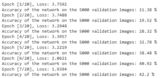
print('Accuracy of the network on the {} validation images: {} %'.format(5000, 100 * correct / total)) We can see the output of the above code as follows which does show that the model is actually learning as the loss is decreasing with every epoch:
Testing
For testing, we use exactly the same code as validation but with the test_loader:
with torch.no_grad():
    correct = 0
    total = 0
    for images, labels in test_loader:
        images = images.to(device)
        labels = labels.to(device)
        outputs = model(images)
        _, predicted = torch.max(outputs.data, 1)
        total += labels.size(0)
        correct += (predicted == labels).sum().item()
        del images, labels, outputs

print('Accuracy of the network on the {} test images: {} %'.format(10000, 100 * correct / total)) Using the above code and training the model for 20 epochs, we were able to achieve an accuracy of 75% on the test set.
Conclusion
Let's now conclude what we did in this article:
- We started by understanding the architecture and different kinds of layers in the VGG-16 model
- Next, we loaded and pre-processed the CIFAR100 dataset using
torchvision - Then, we used
PyTorchto build our VGG-16 model from scratch along with understanding different types of layers available intorch - Finally, we trained and tested our model on the CIFAR100 dataset, and the model seemed to perform well on the test dataset with 75% accuracy
Future Work
Using this article, you get a good introduction and hand-on learning but you'll learn much more if you extend this and see what you can do else:
- You can try using different datasets. One such dataset is CIFAR10 or a subset of ImageNet dataset.
- You can experiment with different hyperparameters and see the best combination of them for the model
- Finally, you can try adding or removing layers from the dataset to see their impact on the capability of the model. Better yet, try to build the VGG-19 version of this model