As a Data Scientist and Researcher, I always try to find answers to the problems I come across every day. Working on real-world problems, I have faced many complexities both in time and computation. There have been many cases where the classical machine learning and deep learning algorithms failed to work, and my computer ended up crashing.
During the lockdown, I stumbled upon a cool new sci-fi series called Devs streaming on Hulu. Devs explores quantum computing and scientific research that is actually happening now, around the world. This led me to think about Quantum Theory, how Quantum Computing came to be, and how Quantum Computers can be used to make future predictions.
After researching further I found Quantum Machine Learning (QML), a concept that was pretty new to me at the time. This field is both exciting and useful; it could help resolve issues with computational and time complexities, like those that I faced. Hence, I chose QML as a topic for further research and decided to share my findings with everyone.
Quantum Machine Learning is a theoretical field that’s just starting to develop. It lies at the intersection of Quantum Computing and Machine Learning.
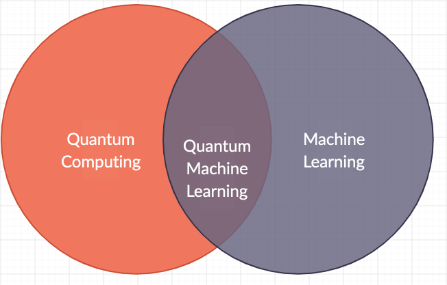
The main goal of Quantum Machine Learning is to speed things up by applying what we know from quantum computing to machine learning. The theory of Quantum Machine Learning takes elements from classical Machine Learning theory, and views quantum computing from that lens.
Contents
This post will cover the following main topics:
- Comparison of Classical Programming with Classical Machine Learning and Quantum Machine Learning
- All the Basic Concepts of Quantum Computing
- How Quantum Computing Can Improve Classical Machine Learning Algorithms
Bring this project to life
Classical Programming vs. Classical Machine Learning vs. Quantum Machine Learning
To compare Classical Programming, Classical Machine Learning, and Quantum Machine Learning, let's consider the simple problem of determining whether a number is even or odd.
The solution is simple enough: first you need to get a number from the user, then you divide the number by two. If you get a remainder, then that number is odd. If you don’t get a remainder, then that number is even.
If you want to write this particular program using the classical programming approach, you would follow three steps:
- Get the input
- Process the input
- Produce the output
This is the workflow of the classical programming paradigm.
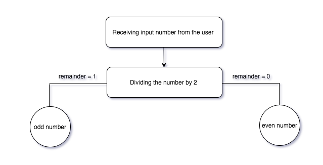
The processing is done through the rules which we have defined for the classification of the number — even or odd.
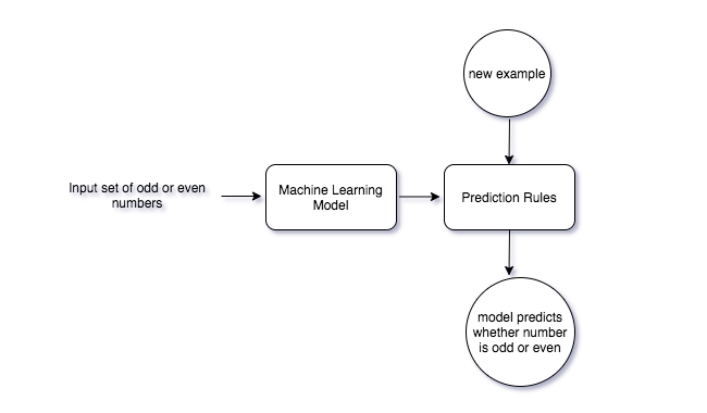
Similarly, let’s look at how we would solve this particular problem using a Machine Learning approach. In this case things are a bit different. First we create a set of input and output values. Here, the approach would be to feed the input and expected output together to a machine learning model, which should learn the rules. With machine learning we don't tell the computer how to solve the problem; we set up a situation in which the program will learn to do so itself.
Mathematically speaking, our aim is to find f, given x and y, such that:
y = f(x)
Let’s move onto Quantum Computing. Whenever you think of the word "quantum," it might trigger the idea of an atom or molecule. Quantum computers are made up of a similar idea. In a classical computer, processing occurs at the bit-level. In the case of Quantum Computers, there is a particular behavior that governs the system; namely, quantum physics. Within quantum physics, we have a variety of tools that are used to describe the interaction between different atoms. In the case of Quantum Computers, these atoms are called "qubits" (we will discuss that in detail later). A qubit acts as both a particle and a wave. A wave distribution stores a lot of data, as compared to a particle (or bit).
Loss functions are used to keep a check on how accurate a machine learning solution is. While training a machine learning model and getting its predictions, we often observe that all the predictions are not correct. The loss function is represented by some mathematical expression, the result of which shows by how much the algorithm has missed the target.
A Quantum Computer also aims to reduce the loss function. It has a property called Quantum Tunneling which searches through the entire loss function space and finds the value where the loss is lowest, and hence, where the algorithm will perform the best and at a very fast rate.
The Basics of Quantum Computing
Before getting deep into Quantum Machine Learning, readers should be familiar with basic Quantum Computing terminologies, which are discussed here.
Bra-ket Notation
In quantum mechanics and quantum physics, the “Bra-ket” notation or “Dirac” notation is used to write equations. Readers (especially beginners) must know about this because they will come across it when they read research papers involving quantum computing.
The notation uses angle brackets, 〈 〉, and a vertical bar, | , to construct “bras” and “kets”.
A “ket” looks like this: |v〉. Mathematically it denotes a vector, v, in a complex vector space V. Physically, it represents the state of a quantum system.
A “bra” looks like this:〈f| . Mathematically, it denotes a linear function f: V → C, i.e. a linear map that maps each vector in V to a number in the complex plane C.
Letting a linear function〈f| act on a vector |v〉is written as:
〈f|v〉⍷ C
Wave functions and other quantum states can be represented as vectors in a complex state using the Bra-ket notation. Quantum Superposition can also be denoted by this notation. Other applications include wave function normalization, and measurements associated with linear operators.
The Concept of “Qubits” and the Superposition States
Quantum Computing uses “qubits” instead of “bits,” which are used by classical computers. A bit refers to a binary digit, and it forms the basis of classical computing. The term “qubit” stands for Quantum Binary Digit. While bits have only two states —0 and 1—qubits can have multiple states at the same time. The value ranges between 0 and 1.
To better understand this concept, take the analogy of a coin toss. A coin has two sides , Heads (1) or Tails (0). While the coin is being tossed, we don't know which side it has until we stop it or it falls on the ground. Look at the coin toss shown below. Can you tell which side it has? It shows both 0 and 1 depending on your perspective; only if you stop it to look does it show just one side. The case with qubits is similar.

This is called the superposition of two states. This means that the probabilities of measuring a 0 or 1 are generally neither 0.0 nor 1.0. In other words, there is a likelihood that the quibit is in various states at once. In the case of the coin toss, when we get our result (heads or tails) the superposition collapses.
The Bloch Sphere
The Bloch Sphere is the mathematical representation of a qubit. It represents the state of a qubit by a two-dimensional vector with a normal length of one. This vector has two elements: a real number α and a complex number β.
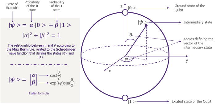
A qubit can be considered as a superposition of two states and can be denoted by the following statement, explained in the image above:
|ψ〉 = α |0〉 + β |1〉
For historical reasons in optics, the Bloch sphere is also known as the Poincaré sphere and specifically represents different types of polarization. Six common polarization types exist, and are called Jones vectors. Indeed, Henri Poincaré was the first to suggest the use of this kind of geometrical representation at the end of the 19th century, as a three-dimensional representation of Stokes parameters.
Quantum Decoherence
The superposition of qubits causes issues like Quantum Decoherence. These are unwanted collapses that happen randomly and naturally because of noise in the system. Ultimately, this leads to errors in computation. If you think that a qubit is in a superposition when it isn't, and we do an operation on it, it’s going to give you a different answer than you might have expected. This is why we run the same program over and over again many times, similar to training a machine learning model.
What Causes Quantum Decoherence?
Quantum systems need to be isolated from the environment, because contact with the environment is what causes quantum decoherence.
Qubits are chilled to near absolute zero. When qubits interact with the environment, information from the environment leaks into them, and information from within the qubits leaks out. The information that leaks out is most likely needed for a future or current computation, and the information that leaks in is random noise.
This concept is exactly like the Second Law of Thermodynamics, which states that:
“The total entropy of an isolated system can never decrease over time, and is constant if and only if all processes are reversible. Isolated systems spontaneously evolve towards thermodynamic equilibrium, the state with maximum entropy.”

Thus, quantum systems need to be in a state of coherence. Quantum decoherence is more visible in minute particles as compared to bigger objects, like a book or a table. It is a fact that all materials have a particular wavelength associated with them, but the bigger the item, the lesser its wavelength.
Quantum Entanglement
The idea of Quantum Entanglement refers to the idea that if we take two qubits, they are always in a superposition of two states. Here’s an example. Suppose there is a box and inside of it, there is a pair of gloves. At random, one glove is taken out of the box. The box is then taken to a different room. The glove that was taken out was found to be right-handed, so we automatically know that the glove that is still inside the box is left-handed.

The same is the case with qubits. If one is in a spin-up position, then the other is automatically in the spin-down position. There does not exist a scenario where both the qubits are in the same state. In other words, they are always entangled. This is known as quantum entanglement.
Dual Principle
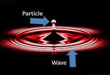
Qubits exhibit properties of both waves and particles. In fact, all objects do, but they can be observed more clearly in atomic-sized objects like the qubit. The wave-particle duality enables qubits to interact with each other by interference.
Quantum Speedup
Quantum Coherence helps the quantum computer to process information in a way that classical computers cannot. A quantum algorithm performs a stepwise procedure to solve a problem, such as searching a database. It can outperform the best known classical algorithms. This phenomenon is called the Quantum Speedup.
How Quantum Computing Can Improve Classical Machine Learning
Now that you're aware of a few basic concepts of Quantum Computing, let's discuss some methods that quantum computers use to solve machine learning problems. The techniques that we are going to look through are listed below:
- Quantum Machine Learning to Solve Linear Algebraic Problems
- Quantum Principal Component Analysis
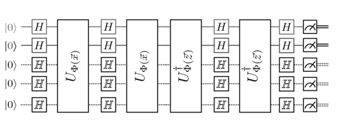
- Quantum Support Vector Machines and Kernel methods
- Quantum Optimization
- Deep Quantum Learning
1) Quantum Machine Learning to Solve Linear Algebraic Problems
A wide variety of Data Analysis and Machine Learning problems are solved by performing matrix operation on vectors in a high dimensional vector space.
In quantum computing, the quantum state of the qubits is a vector in a 2ª-dimensional complex vector space. A lot of matrix transformations happen in this space. Quantum Computers can solve common linear algebraic problems such as the Fourier Transformation, finding eigenvectors and eigenvalues, and solving linear sets of equations over 2ª-dimensional vector spaces in time that is polynomial in a (and exponentially faster than classical computers due to the Quantum Speedup). One of the examples is the Harrow, Hassidim, and Lloyd (HHL) algorithm.

2) Quantum Principal Component Analysis
Principal Component Analysis is a dimensionality reduction technique that is used to reduce the dimensionality of large datasets. Dimensionality reduction comes at the cost of accuracy, as we need to decide which variables to eliminate without losing important information. If done correctly, it makes the machine learning task much more comfortable because it is more convenient to deal with a smaller dataset.
For instance, if we have a dataset that has ten input attributes, then principal component analysis can be carried out efficiently by a classical computer. But if the input dataset has a million features, the classical methods of principal component analysis will fail because it will be hard for us to visualize the importance of each variable.
Another issue with classical computers is the calculation of eigenvectors and eigenvalues. The higher the dimensionality of the input, the larger the set of corresponding eigenvectors and eigenvalues. Quantum Computers can solve this problem very efficiently and at a very high speed by using Quantum Random Access Memory (QRAM) to choose a data vector at random. It maps that vector into a quantum state using qubits.
The summarized vector that we get after Quantum Principal Component Analysis has logarithmic qubits. The chosen random vector forms a dense matrix. This matrix is actually the covariance matrix.
By repeatedly sampling the data and using a trick called density matrix exponentiation, combined with the quantum phase estimation algorithm (which calculates the eigenvectors and eigenvalues of the matrices), we can take the quantum version of any data vector and decompose it into its principal components. Both the computational complexity and time complexity is thus reduced exponentially.

3) Quantum Support Vector Machines
Support Vector Machine is a classical Machine learning algorithm used both for classification and regression. For classification tasks it is used to classify linearly separable datasets into their respective classes. Suppose, if the data is not linearly separable, then it’s dimensions are increased till it is linearly separable.
In classical computers, SVM can be performed only up to a certain number of dimensions. After a particular limit, it will be hard because such computers do not have enough processing power.
Quantum Computers, however, can perform Support Vector Algorithm at an exponentially faster rate. The principle of Superposition and entanglement allows it to work efficiently and produce results faster.
4) Quantum Optimization
If you are trying to produce the best possible output by using the least possible resources, it is called optimization. Optimization is used in a machine learning model to improve the learning process so that it can provide the most adequate and accurate estimations.
The main aim of optimization is to minimize the loss function. A more considerable loss function means there will be more unreliable and less accurate outputs, which can be costly and lead to wrong estimations.
Most methods in machine learning require iterative optimization of their performance. Quantum optimization algorithms suggest improvement in solving optimization problems in machine learning. The property of quantum entanglement enables to produce multiple copies of the present solution, encoded in a quantum state. They are used to improve that solution at each step of the machine learning algorithm.
5) Deep Quantum Learning
Quantum computing can be combined with deep learning to reduce the time required to train a neural network. By this method, we can introduce a new framework for deep learning and performing underlying optimization. We can mimic classical deep learning algorithms on an actual, real-world quantum computer.
When multi-layer perceptron architectures are implemented, the computational complexity increases as the number of neurons increases. Dedicated GPU clusters can be used to improve the performance, significantly reducing training time. However, even this will increase when compared with quantum computers.
Quantum Computers itself are designed in such a way where the hardware can mimic the neural network instead of the software used in classical computers. Here, a qubit acts as a neuron that constitutes the basic unit of a neural network. Hence, a Quantum System which contains qubits can act as a neural network and can be used for deep learning applications at a rate that surpasses any classical machine learning algorithm.
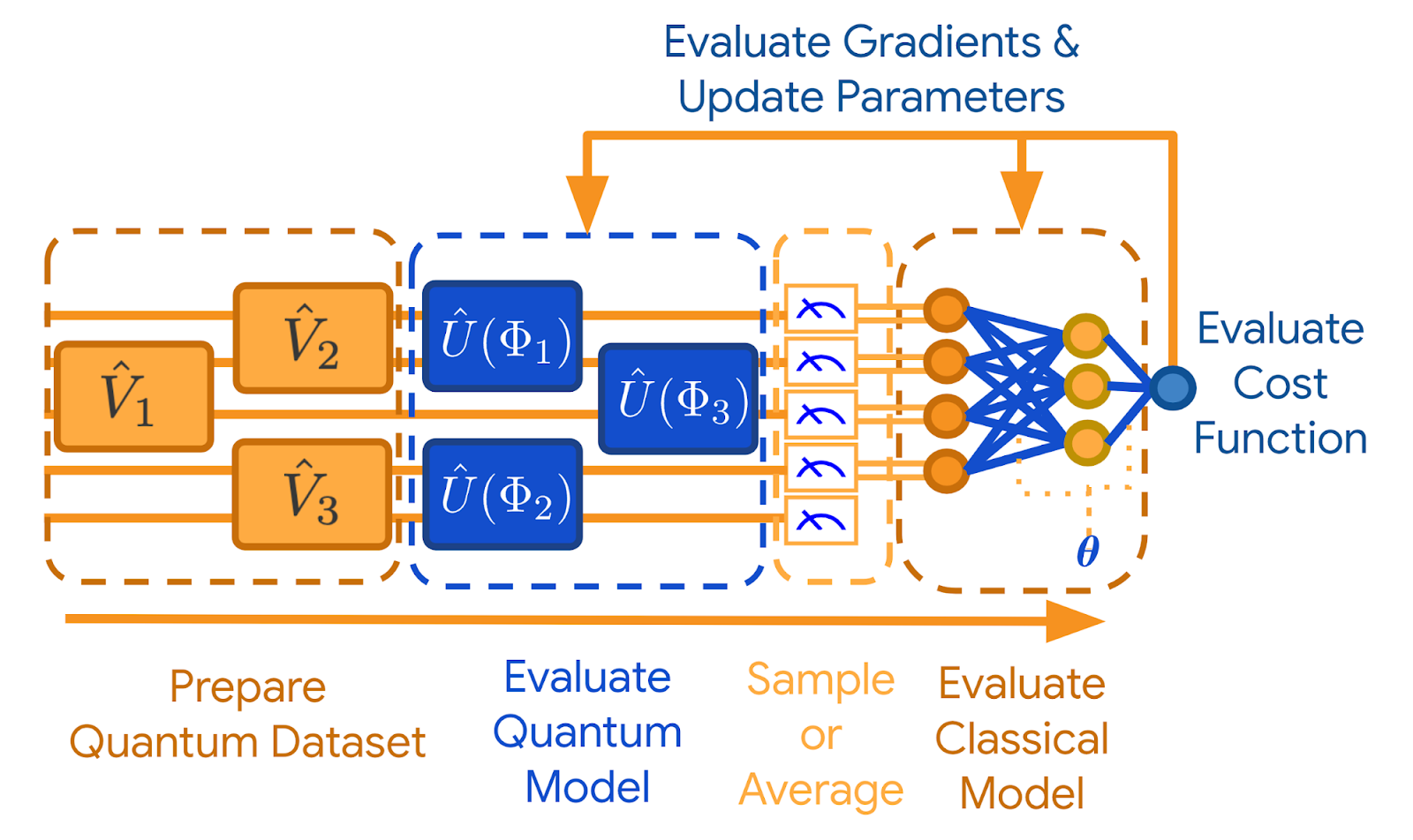
Simulation of Quantum Machine Learning
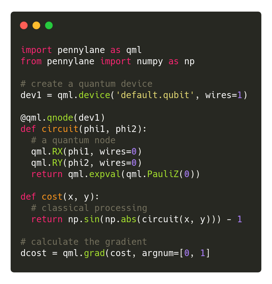
PennyLane is an open-source software from Xanadu for performing simulations of Quantum Machine learning. It combines classical machine learning packages with quantum simulators and hardware.
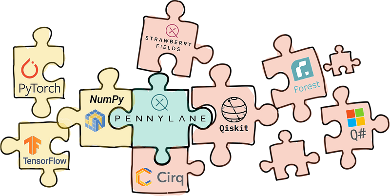
PennyLane supports a growing ecosystem, including a wide range of quantum hardware and machine learning libraries.
“While the community is still working towards fault-tolerant quantum computing, PennyLane and hardware offerings, allow enterprise clients to start leveraging quantum computing today”
— Nathan Killoran, Head of Software and Algorithms at Xanadu.
Conclusion
In this article we looked at the basics of Quantum Computing, which can be used to implement Machine Learning.
Quantum Machine Learning is a growing field, and researchers say that by the mid-2030s Quantum Computers will become popular, and people will start using them.
Here, we first compared Classical Programming with Classical Machine Learning and Quantum Machine Learning. We found Quantum Machine Learning Algorithms to be the best amongst them.
Then, we took a deep dive into the basics of Quantum Computing. We discussed:
- The bra-ket notation, which is used to write equations in quantum physics.
- The concept of qubits and the Superposition theorem that governs the state of the qubits.
- The Bloch’s sphere, which is used to represent the state of a qubit, Mathematically
- The Quantum Decoherence and its cause
- The Quantum Entanglement with an example
- The Dual principle of objects
- The Quantum Speedup
Now that the readers were familiar with the basic quantum computing terminologies, we looked into ways how Quantum Computing could enhance Classical Machine Learning by using the following methods:
- Quantum Machine Learning to solve Linear Algebraic problems,
- Quantum Principal Component Analysis,
- Quantum Support Vector Machines and Kernel methods,
- Quantum Optimization, and
- Deep Quantum Learning.
In all these techniques, we looked into how Quantum Systems worked better than a classical system.
We also saw and learned briefly about PennyLane, an open-source software that is used in the simulation of Quantum Machine Learning Algorithms.
In short, the future of quantum computing will see us solving some of the most complex questions facing the world today.
There’s a huge opportunity for quantum machine learning to disrupt a number of industries. The financial, pharmaceutical, and security industries will see the most change in the shortest amount of time.
While some experts have warned that this power could be used for dangerous purposes, William Hurley, chair of the Quantum Computing Standards Workgroup at the Institute of Electrical and Electronics Engineers (IEEE) believes the good will outweigh the bad. According to him:
“There will always be reasons to temper our optimism around any new technological advance. Still, I am incredibly excited about the potential positive outcomes of quantum computing. From finding new cures to diseases to helping discover new particles, I think this is the most excited I have been in my entire career. We should be focusing our energy as much on the positive outcomes as we currently are the negative ones.”
In other words, Quantum Machines can lead us to a better life and if used effectively, can eradicate a lot of hurdles on our way to enhancing Machine Learning Algorithms.
References
This article is a result of research from various sources and are listed below:


