BERT Transformers for Natural Language Processing

The magnificence of artificial intelligence, especially in the sub-domain of deep learning, has been consistently advancing, with numerous achievements every month as progress races forward. Many of my articles have been primarily focused on two significant subdomains of deep learning: namely computer vision and natural language processing (NLP). NLP focuses on linguistic tasks, grammar, and semantic understanding of a language. We utilize deep learning models to ensure that we can come up with a pattern for the AI to decode the intricate details and particular patterns of the specific context of text or sentences. To that end, there have been many methods developed since the inception of the field that aim to solve some of the major NLP problems, such as text classification, translation of languages (machine translation), chatbots, and other similar tasks.

Some of the popular methods to solve these kinds of tasks include the sequence-to-sequence models, the utility of attention mechanisms, transformers, and other similar popular techniques. In this article, our primary focus is one of the more successful variations of transformers, Bidirectional Encoder Representations from Transformers (BERT). We will understand most of the essential concepts required to get started and also utilize this BERT architecture to compute solutions for natural language processing problems. The table of contents below shows the list of features we will discuss in this blog post. For running the code alongside, I would recommend making use of the Gradient platform on Paperspace.

Introduction:

Most of the tasks related to natural language processing were initially solved with the help of simple LSTMs (long-short term memory) networks. These layers would be stacked upon each other to yield the learning process of vector words. However, these networks alone weren't sufficient to produce high-quality results and failed in tasks and projects requiring more precision, such as neural machine translation and text classification tasks. The primary reason for this failure of simple LSTMs is that they are slow and clunky networks. Also, no variation of LSTM is fully bidirectional. Hence, the context and the true meaning of the word vectors are lost as we move ahead in the learning process.

One of the groundbreaking revolutions in these tasks occurred in the year 2017 with the introduction of transformers. These transformer networks published in the "Attention is all you need" research paper revolutionized the world of natural language processing with its unique approach to combat the previously existing issues with simple LSTM architectures. In one of my previous articles, we have covered the concept of transformers in extreme detail. I would highly recommend checking out this blog from the following link. We will learn that there is a close relationship between the transformer networks and the BERT architecture further in the upcoming section.

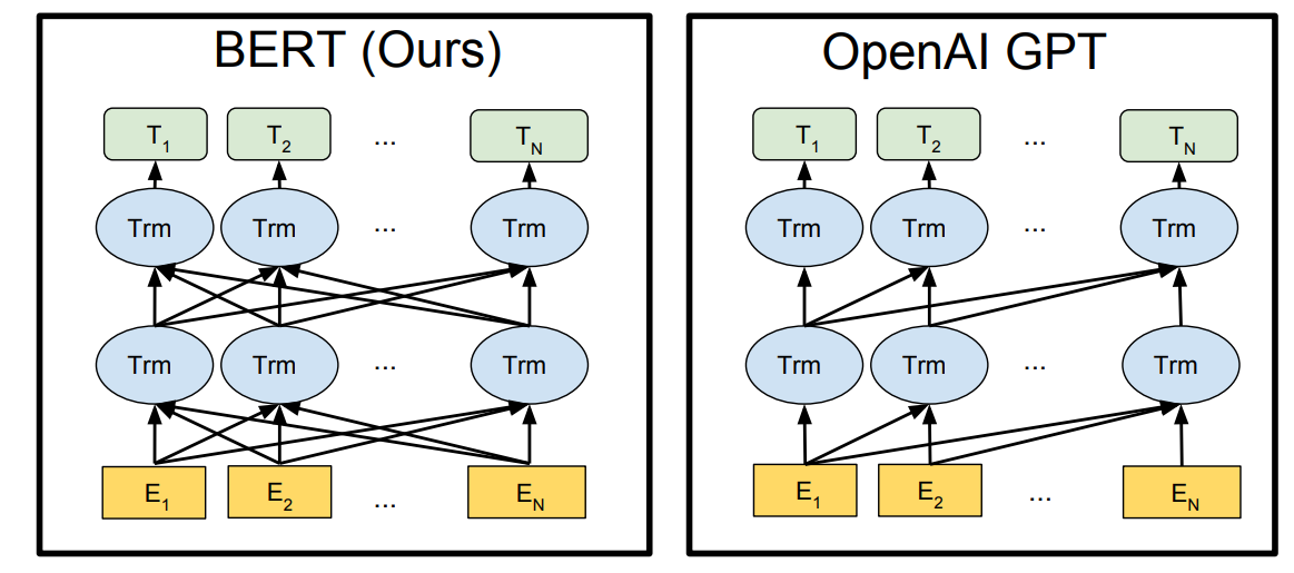
However, for now, it is significant to note that when we stack a bunch of decoder layers of the transformer network while ignoring the encoder network of the transformers, we will obtain the Generative Pre-trained Transformer (GPT) models. This popular architecture has had a couple more variations with the GPT-2 and GPT-3 networks, constantly improving with each of its previous versions. However, if we disregard the decoder networks of the transformer and stack the encoder section of the transformer models, we will obtain the Bidirectional Encoder Representations from Transformers (BERT). In the upcoming section, we will go into greater detail and understand the working mechanism of the BERT transformers through which we can solve numerous problems with ease.

Understanding BERT Transformers:

Unlike simple LSTM networks, BERT transformers are capable of understanding language in fair more complex manners. In a transformer architecture, both the individual encoder network and decoder blocks have the capability to understand language. Hence, the stacking of either of these layers results in a scenario where the produced networks are capable of understanding and learning a language. But, the question arises on how exactly are these BERT models trained and utilized for performing a variety of natural language processing tasks.

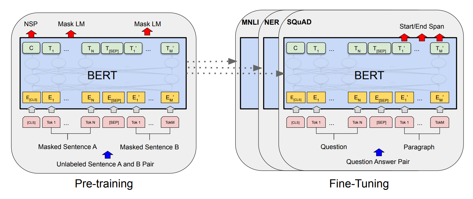
The training process of BERT is comprised of mainly two phases, namely the pre-training of the BERT model and fine-tuning of the BERT model. In the pre-training step, our primary objective is to teach our BERT model an understanding of the language. This process is done by using a semi-supervised learning approach: training the data on large amounts of information gathered from across the web or other resources. In the pre-training step of the BERT model, two tasks are run simultaneously, which include Masked Language Model (MLM) and Next Sentence Prediction (NSP) to understand the context (or language).

In Masked Language Models (MLM), we make use of masks to hide some of the data in the sentences (about 15%) to make the model understand the context of the sentences better. The goal is to output these masked tokens to achieve the desired language understanding by utilizing bidirectionality. In the case of the Next Sentence Prediction (NSP), the BERT model considers two sentences and determines if the second sentence is an appropriate follow-up to the first sentence.

With the help of pre-training, the BERT model is able to achieve an understanding of context and language. However, to use it for the specific task that we are trying to perform, we require the second step of fine-tuning. In fine-tuning the BERT model, we replace the fully connected output layers with our new network of layers. The fine-tuning step of the BERT model is a supervised learning task, where we train the model to accomplish the particular task.

Since the network is already pre-trained, the fine-tuning step will be relatively faster as only the new network has to be trained, while the other weights are slightly modified (fine-tuned) accordingly for the specific project. We will discuss what these specific tasks are in the application section of this article. For now, let us proceed to develop a review score classification project with BERT.

Developing a project with BERT using TensorFlow-Hub:

In this section of the article, we will explore a detailed breakdown of how to load a pre-trained BERT model available from TensorFlow Hub and add additional transfer learning layers to this BERT model to construct a project for text classification. We will utilize the TensorFlow and Keras deep learning frameworks for this article. I would highly recommend checking out both of these libraries from my previous blogs if you aren't familiar with them or to quickly brush up on these topics. You can check out the following article to learn more about TensorFlow and the Keras article here. Let us get started with the creation of the BERT working pipeline by importing the necessary libraries.

Importing the required libraries:

The TensorFlow deep learning framework, along with the TensorFlow Hub imports, is quintessential to this project. The TensorFlow Hub library enables developers to load pre-trained models for further fine-tuning and deployment of numerous projects. We will also import some additional layers that we will add to the pooled output layer of the BERT model, and use these changes to create a transfer learning model for performing a text classification task.

We will also use some additional callbacks for saving the trained model and visualizing the performance with the Tensor board. Also, some other basic imports such as the NumPy library, the os library to access the system components, re for regulating regular expression operations, and warnings to filter out unnecessary comments are used.

#Importing the essential libraries

import tensorflow as tf
import tensorflow_hub as hub
from tensorflow.keras.models import Model
from tensorflow.keras.layers import Input, Dense, Activation, Dropout, Flatten
from tensorflow.keras.layers import BatchNormalization, Conv2D, MaxPool2D
from tensorflow.keras.models import Model, Sequential
from tensorflow.keras.callbacks import ModelCheckpoint, ReduceLROnPlateau
from tensorflow.keras.callbacks import LearningRateScheduler, TensorBoard
from datetime import datetime
from sklearn.metrics import roc_auc_score
import numpy as np
import pandas as pd
from tqdm import tqdm
import os
import re
import warnings
warnings.filterwarnings("ignore")

Preparing the dataset:

We will utilize the Amazon Fine Food Reviews dataset that can be obtained from the following Kaggle link. Below is a brief description of the dataset and its corresponding code snippet to read and understand the data. Ensure that the file is placed in the working directory where you are constructing the project.

This dataset consists of reviews of fine foods from amazon. The data span a period of more than 10 years, including all ~500,000 reviews up to October 2012. Reviews include product and user information, ratings, and a plain text review. It also includes reviews from all other Amazon categories.
- Kaggle

#Read the dataset - Amazon fine food reviews
reviews = pd.read_csv("Reviews.csv")

#check the info of the dataset
reviews.info()

In the next step, we will filter out any of the unnecessary "not a number" (NAN) values while retrieving only the text information and their respective scores.

# Retrieving only the text and score columns while drop NAN values

reviews = reviews.loc[:, ['Text', 'Score']]
reviews = reviews.dropna(how='any')
reviews.head(1)

In the next step, we will convert the scores of the text data into a binary classification task with only negative or positive reviews by omitting the neutral scores. The neutral scores, i.e., the scores with a value of three, are removed. Since this is a binary classification task on natural language processing, we are trying to avoid neutral reviews. All scores with a value less than two are considered to be negative reviews, and all scores with a value greater than three are considered to be positive reviews.

reviews.loc[reviews['Score'] <= 2, 'Score'] = 0 
reviews.loc[reviews['Score'] > 3, 'Score'] = 1
reviews.drop(reviews[reviews['Score']==3].index, inplace=True)
        
reviews.shape

(525814, 2)

In the next step, we will perform some required pre-processing for the dataset. We will create two functions. The first function will enable us to retrieve only the first fifty words, and the second function will allow us to remove some of the unnecessary characters that are not required for the training process. We can call the function and obtain the new dataset. Below is the code block and the sample dataset after pre-processing.

def get_wordlen(x):
    return len(x.split())
reviews['len'] = reviews.Text.apply(get_wordlen)
reviews = reviews[reviews.len<50]
reviews = reviews.sample(n=100000, random_state=30)

def remove_html(text):
    html_pattern = re.compile('<.*?>')
    return html_pattern.sub(r'', text)

text=reviews['Text']
preprocesstext=text.map(remove_html)
reviews['Text']=preprocesstext

#print head 5
reviews.head(5)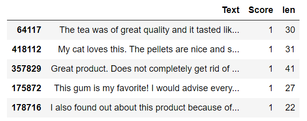

Below is the code block for splitting the data with a stratified sampling and a specific random state. Stratified sampling splits allow us to maintain a balanced count of 0's and 1's in both the train and test data, i.e., an adequate binary composition is maintained. The random state specification allows us to track results easier in a non-varied manner across various systems and platforms. Below is the code snippet for splitting the dataset and its respective training and testing plots.

# Split the data into train and test data(20%) with Stratify sampling and random state 33 

from sklearn.model_selection import train_test_split
X = reviews['Text']
y = reviews["Score"].values
X_train, X_test, y_train, y_test = train_test_split(X, y, test_size=0.20, stratify=y, random_state = 33)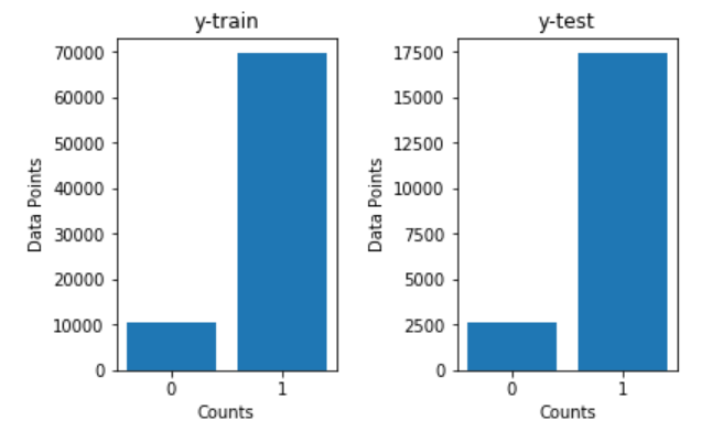

Finally, after all the steps performed in this section, you can proceed to save the data to the working directory in the form of a pre-processed CSV file to further any further computations if required.

# Saving to disk. if we need, we can load preprocessed data directly. 
reviews.to_csv('preprocessed.csv', index=False)

Developing the BERT Model:

For this project, we will make use of the BERT uncased model, which you can acquire from the following TensorFlow Hub website. It uses L=12 hidden layers (i.e., Transformer blocks), a hidden size of H=768, and A=12 attention heads. As discussed in the previous section, while using the pre-trained BERT model, we will also pass a masked input. We can retrieve the desired output from the BERT model and proceed to perform further transfer learning operations on it.

## Loading the Pretrained Model from tensorflow HUB
tf.keras.backend.clear_session()

max_seq_length = 55

# Creating the necessary requirements
input_word_ids = tf.keras.layers.Input(shape=(max_seq_length,), dtype=tf.int32, name="input_word_ids")
input_mask = tf.keras.layers.Input(shape=(max_seq_length,), dtype=tf.int32, name="input_mask")
segment_ids = tf.keras.layers.Input(shape=(max_seq_length,), dtype=tf.int32, name="segment_ids")

#bert layer 
bert_layer = hub.KerasLayer("https://tfhub.dev/tensorflow/bert_en_uncased_L-12_H-768_A-12/1", trainable=False)
pooled_output, sequence_output = bert_layer([input_word_ids, input_mask, segment_ids])

bert_model = Model(inputs=[input_word_ids, input_mask, segment_ids], outputs=pooled_output)
bert_model.summary()

Model: "model"
__________________________________________________________________________________________________
 Layer (type)                   Output Shape         Param #     Connected to                     
==================================================================================================
 input_word_ids (InputLayer)    [(None, 55)]         0           []                               
                                                                                                  
 input_mask (InputLayer)        [(None, 55)]         0           []                               
                                                                                                  
 segment_ids (InputLayer)       [(None, 55)]         0           []                               
                                                                                                  
 keras_layer (KerasLayer)       [(None, 768),        109482241   ['input_word_ids[0][0]',         
                                 (None, 55, 768)]                 'input_mask[0][0]',             
                                                                  'segment_ids[0][0]']            
                                                                                                  
==================================================================================================
Total params: 109,482,241
Trainable params: 0
Non-trainable params: 109,482,241
__________________________________________________________________________________________________

Once we have acquired the pre-trained BERT model, we can proceed to do some final tokenization on the available data as well as develop the final model that will be fine-tuned to contribute toward the specific task we are aiming to achieve.

Tokenization:

In the next step, we will perform the tokenization action on the dataset. For computing this specific action, it is essential to download a pre-processing file titled tokenization.py from the following official GitHub link (use wget on the raw file using the terminal in Gradient). Once we have downloaded the following file and placed it in the working directory, we can import it to our main project file. In the code block below, we convert the larger data into smaller chunks of useful and understandable information for the BERT model.

We tokenize the reviews and the [CLS] (classification) and [SEP] (Separators) operation at the start and end of the tokens, respectively. Doing so will help the BERT model to differentiate between the start and end of each sentence, often useful in binary classification or next sentence prediction projects. We can also add some additional padding to avoid shape mismatches, and finally, proceed to create the training and testing data as shown in the below code block.

#getting Vocab file
vocab_file = bert_layer.resolved_object.vocab_file.asset_path.numpy()
do_lower_case = bert_layer.resolved_object.do_lower_case.numpy()

#import tokenization from the GitHub link provided
import tokenization

tokenizer = tokenization.FullTokenizer(vocab_file, do_lower_case)

X_train=np.array(X_train)
# print(X_train[0])
X_train_tokens = []
X_train_mask = []
X_train_segment = []
X_test_tokens = []
X_test_mask = []
X_test_segment = []

def TokenizeAndConvertToIds(text):
    tokens= tokenizer.tokenize(reviews) # tokenize the reviews
    tokens=tokens[0:(max_seq_length-2)] 
    tokens=['[CLS]',*tokens,'[SEP]'] # adding cls and sep at the end
    masked_array=np.array([1]*len(tokens) + [0]* (max_seq_length-len(tokens))) # masking 
    segment_array=np.array([0]*max_seq_length)
    if(len(tokens)<max_seq_length):
        padding=['[PAD]']*(max_seq_length-len(tokens)) # padding
        tokens=[*tokens,*padding]
    tokentoid=np.array(tokenizer.convert_tokens_to_ids(tokens)) # converting the tokens to id
    return tokentoid,masked_array,segment_array

for reviews in tqdm(X_train):
    tokentoid,masked_array,segment_array=TokenizeAndConvertToIds(reviews)
    X_train_tokens.append(tokentoid)
    X_train_mask.append(masked_array)
    X_train_segment.append(segment_array)
    
for reviews in tqdm(X_test):
    tokentoid,masked_array,segment_array=TokenizeAndConvertToIds(reviews)
    X_test_tokens.append(tokentoid)
    X_test_mask.append(masked_array)
    X_test_segment.append(segment_array)
    
X_train_tokens = np.array(X_train_tokens)
X_train_mask = np.array(X_train_mask)
X_train_segment = np.array(X_train_segment)
X_test_tokens = np.array(X_test_tokens)
X_test_mask = np.array(X_test_mask)
X_test_segment = np.array(X_test_segment)

Once you have successfully created all the tokens, it might be a good idea to save them in a pickle file to reload them for any required future computations. You can do so from the code snippet below, which shows both the dumping and loading functionalities.

import pickle

# save all your results to disk so that, no need to run all again. 
pickle.dump((X_train, X_train_tokens, X_train_mask, X_train_segment, y_train),open('train_data.pkl','wb'))
pickle.dump((X_test, X_test_tokens, X_test_mask, X_test_segment, y_test),open('test_data.pkl','wb'))

# you can load from disk
X_train, X_train_tokens, X_train_mask, X_train_segment, y_train = pickle.load(open("train_data.pkl", 'rb')) 
X_test, X_test_tokens, X_test_mask, X_test_segment, y_test = pickle.load(open("test_data.pkl", 'rb')) 

Training a transfer learning model on BERT:

Once we have completed the pre-processing of the data, pre-training the BERT model, and tokenization of the data, we can proceed to create the transfer learning model by developing our fine-tuned architecture model. Firstly, let us obtain the output for the training data by passing the tokens, masks, and their respective segments.

# get the train output with the BERT model
X_train_pooled_output=bert_model.predict([X_train_tokens,X_train_mask,X_train_segment])

Similarly, we will perform the prediction with the BERT model on the test data as well, as shown in the below code snippet.

# get the test output with the BERT model
X_test_pooled_output=bert_model.predict([X_test_tokens,X_test_mask,X_test_segment])

In the next step, we can use the pickle library to store the predictions. Note that the previous two prediction steps can take a little time to run, depending on your system hardware. Once you have successfully saved the prediction outputs and dump them in a pickle file, you comment the statement out. You can then use the pickle library again to load the data for any future computations.

# save all the results to the respective folder to avoid running the previous predictions again. 
pickle.dump((X_train_pooled_output, X_test_pooled_output),open('final_output.pkl','wb'))

# load the data for second utility
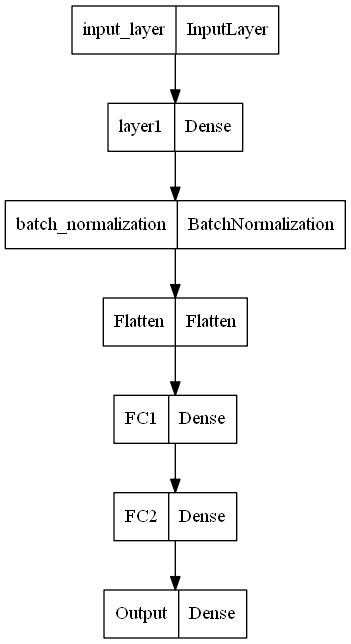
X_train_pooled_output, X_test_pooled_output= pickle.load(open('final_output.pkl', 'rb'))

We will create a custom architecture that we can add to the pre-trained BERT model as the fine-tuning layers. We will add an input layer with 768 input features, a dense layer which the specified parameters, a batch normalization layer, and a flattened layer. We will finally use three back-to-back fully connected layers to complete the network.

The final output layer will make use of the sigmoid activation function with one output node as it is a binary classification task, and we need to predict if the resulting output is positive or negative. I have used the functional API type modeling to allow for more control over the layers and architectural build. The Sequence modeling structure can also be utilized instead in this step.

# input layer
input_layer=Input(shape=(768,), name='input_layer') 

# Dense layer
layer1 = Dense(50,activation='relu',kernel_initializer=tf.keras.initializers.RandomUniform(0,1), name='layer1')(input_layer) 

# MaxPool Layer
Normal1 = BatchNormalization()(layer1)

# Flatten
flatten = Flatten(data_format='channels_last',name='Flatten')(Normal1)

# FC layer
FC1 = Dense(units=30,activation='relu',kernel_initializer=tf.keras.initializers.glorot_normal(seed=32),name='FC1')(flatten)

# FC layer
FC2 = Dense(units=30,activation='relu',kernel_initializer=tf.keras.initializers.glorot_normal(seed=33),name='FC2')(FC1)

# output layer
Out = Dense(units=1,activation= "sigmoid", kernel_initializer=tf.keras.initializers.glorot_normal(seed=3),name='Output')(FC2)

model = Model(inputs=input_layer,outputs=Out)

Once the transfer learning fine-tuned model is created, we can call some essential callbacks to save our model and monitor the results accordingly. However, a few of these callbacks might not be necessary as the training process is quite fast. We will monitor the AUROC score for this model as it represents a more accurate description of the result obtained.

checkpoint = ModelCheckpoint("best_model1.hdf5", monitor='accuracy', verbose=1,
    save_best_only=True, mode='auto', save_freq=1)

reduce = ReduceLROnPlateau(monitor='accuracy', factor=0.2, patience=2, min_lr=0.0001, verbose = 1)

def auroc(y_true, y_pred):
    return tf.py_function(roc_auc_score, (y_true, y_pred), tf.double)

logdir = os.path.join("logs", datetime.now().strftime("%Y%m%d-%H%M%S"))
tensorboard_Visualization = TensorBoard(log_dir=logdir, histogram_freq=1)

Finally, we can compile and train the model. For the compilation, we will make use of the Adam optimizer, the binary cross-entropy loss, and the accuracy and AUROC metrics. We will train the model for ten epochs with a batch size of 300 and the necessary callbacks as mentioned in the below code block.

model.compile(optimizer='adam', loss='binary_crossentropy', metrics=['accuracy', auroc])

model.fit(X_train_pooled_output, y_train, 
          validation_split=0.2, 
          epochs=10, 
          batch_size = 300,
          callbacks=[checkpoint, reduce, tensorboard_Visualization])

Below is a plot of the model that we have constructed for a better conceptual understanding. This network is constructed on top of the BERT architecture as the fine-tuning step to perform the specific task of text classification.

tf.keras.utils.plot_model(
    model, to_file='model1.png', show_shapes=False, show_layer_names=True,
    rankdir='TB', expand_nested=False, dpi=96
)

In the next step, we will visualize the performance of the training process of the model. We will use magic functions with the tensor board and specify the path to our logs folder stored in the current working directory. We can view a variety of graphs when we run the external tensor board extension. However, we are concerned about the AUROC score as it represents a mostly accurate description of the performance of our model. Below is the graph for the following task.

%load_ext tensorboard

%tensorboard --logdir logs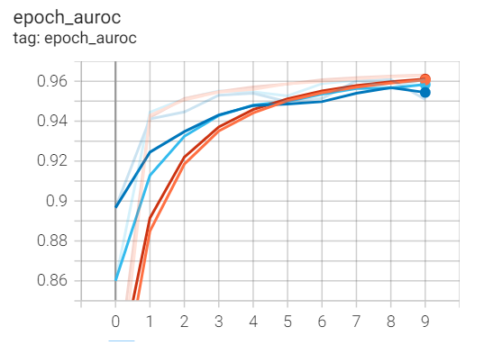

I would recommend trying out numerous iterations and variations of the BERT models to see which type of model suits your particular use case the best. In this section, we discussed how to use the BERT model to solve a binary text classification problem. But, the applications of BERT are not limited to this task. In the upcoming section, we will further explore some more applications of BERT.

Applications of BERT:

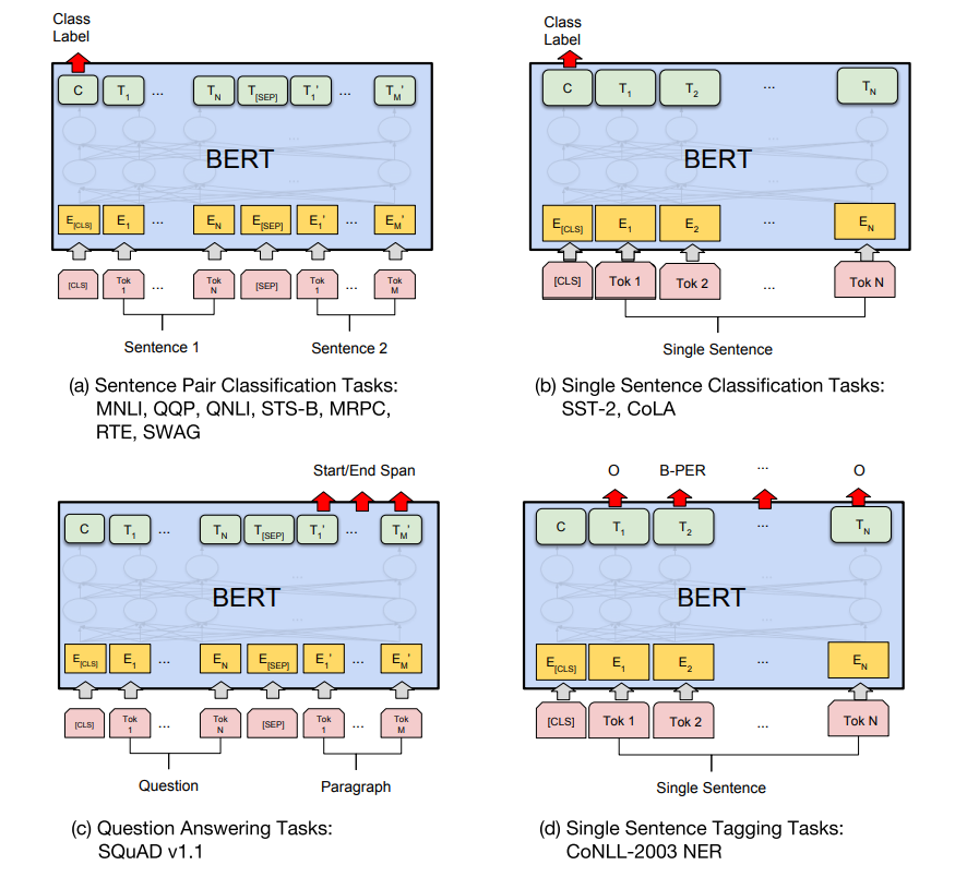
There are numerous applications of the BERT transformer. To summarize how these networks work, we have a pre-trained BERT model that can be utilized to solve a variety of tasks. In the second step, we add the fine-tuning layers that will determine the type of task or application we are trying to perform with the help of the BERT model. Let us look at some of the more popular applications of BERT:

1. Text Classification - In this article, we discuss how we can use the BERT transformer for text classification. The final BERT model was fine-tuned accordingly with the final sigmoid activation function to produce a binary classification output for any given sentence.
2. Question Answering tasks - We can also perform question-answer searches with the BERT model. The [CLS] and [SEP] tokens can be used at the start and end of a question, while the other paragraphs represent the answer. We can train the model accordingly to perform such tasks.
3. Neural Machine Translation - The BERT model is also useful for the task of machine translation, where the architecture can be utilized to translate the information input in one language to another language. We can train the model with specific language inputs to their appropriate translated outputs.
4. Sentiment Analysis - Similar to text classification, we can use the BERT model to classify a variety of emotions. We can classify emotions such as positive, negative, or neutral, as well as extend to some of the other emotions exhibited by humans with the correct context of data to perform such a project.

Apart from these four primary applications, there are numerous more natural language processing applications in which the BERT model can be utilized to achieve desirable results. The field is humungous, with a wide variety of tasks and projects to work on. I would recommend the viewers check out more applications and experiment with the ones already mentioned in this article.

Conclusion:

With the steep rise of social media, the power of artificial intelligence, especially in the branch of deep learning, is at an all-time high. The requirement for these deep learning models to produce and compute effective solutions to solve NLP problems is critical for companies to improve their products. While it was hard to combat and tackle tasks related to NLP in the early ages of deep learning with simple LSTM architectures, there was a revolutionary period during the 2017s and 2018s with the introduction of the transformer networks. In this era, multiple language models were built to produce highly effective results, including the BERT model.

In this article, we had a brief history of NLP with deep learning before proceeding to explain the working concepts behind the working of Bidirectional Encoder Representations from Transformers (BERT). We examined the detailed mechanism of their functionality, and then proceeded to look at the type of natural language processing tasks that these models can perform best. With a basic understanding of the BERT architecture, we then constructed a BERT model with the help of TensorFlow-Hub to perform the task of text classification, producing extremely good results. Finally, we broke down some of the most significant applications of BERT that the modern industry utilizes to achieve high-quality results.

In future articles, we will look at some more effective methods for solving problems and projects related to natural language processing with deep learning. We will also look at other projects based on generative adversarial networks with Cycle GANs, as well as dive deeper into the construction of neural networks from scratch in part 2. Until then, enjoy learning and programming AI projects!

You can create a Gradient Notebook with all the code featured in this blog post by pasting this URL into the "Workplace URL" field in the advanced settings portion of the Gradient Notebook creation page.