Hi folks, welcome to the third part of the GauGAN series. In the last two parts we've covered the components and losses of GauGAN, and how to set up custom training with it. In this part, we'll cover:
- Evaluating the results of GauGAN
- How GauGAN performs compared to its adversaries
We'll close this series with a discussion of how to debug training, and deciding if GauGAN is right for you.
The code in this tutorial is available on the ML Showcase, and you can run it on a free GPU to follow along.
Launch Project For Free
So, let's get started!
Evaluation of GauGAN: Why Is It So Hard?
One of the hardest things about working with GANs is their evaluation. Tasks like object detection and image classification generally predict a finite set of labels, like object class or bounding box coordinates, which make it easy to define the ideal predictions. For example, an ideal prediction for an object detection task would be when all of the predicted bounding boxes are perfectly aligned with the pre-defined class labels. This in turn makes it easy for us to design a loss function that penalizes deviations from the ideal behavior.
Now consider doing the same for GauGAN. The inputs to GauGAN are a latent vector and a semantic segmentation map. How does one define what's expected out of a randomly sampled latent vector? For a semantic segmentation map, we could say that the ideal behavior of GauGAN would be to completely recreate the ground truth image. However, there are a couple of problems with this approach.
For one, let's assume we actually go with some image distance metric like squared distance between the image produced by GauGAN and the real image. Consider a scenario where GauGAN randomly changes the colors of the cars present in the image. The squared distance between the two images will be non-zero due to the different pixels of the cars.
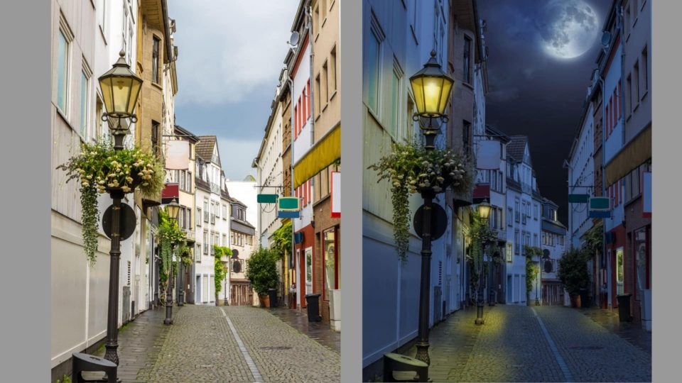
Similarly, consider the following image.

These two images are realistic renditions of the same scene in day and at night (excuse the super moon though). Both of these will have the same originating semantic segmentation map. Let's say the day image is our ground truth, and the night image is what our GAN produced. Since the colors are darker in the latter, the pixels are different and the image would also be interpreted as different. A per-pixel squared distance metric would harshly penalize the dark image, while giving zero error if the GAN produced another day image. While both of these images are equally favorable, we see a squared distance totally fails to recognize this.
Diversity of Samples
Continuing from above, we can say that our squared distance metric is punishing diversity in our image generation, i.e. if we produce realistic but different-looking samples. In fact, image diversity is one of the most fundamental requirements of data generation. If we are just producing the data that we already have, it defeats the purpose of data generation in the first place.
So what is the solution? Well, the best solution is human-level evaluation. As time consuming as it may seem, this is currently the best way to evaluate GANs, and almost all state of the art papers on image generation report this metric.
Human-Level Studies
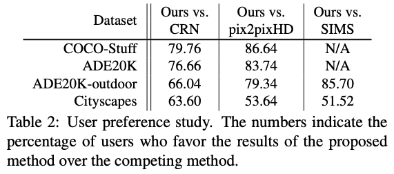
The GauGAN paper uses human-level evaluation to claim its superiority over its contemporaries, like Pix2PixHD, CRN and SIMS.
The test is called a "user-preference study". A set of users are shown two images, one produced by GauGAN and another by the algorithm it's being compared to. The user is then asked which image is more realistic. The percentage by which users prefer GauGAN's image is known as its preference percentage.
GauGAN, primarily because of SPADE, fares much better than its predecessor Pix2PixHD.
We can look at some images ourselves.
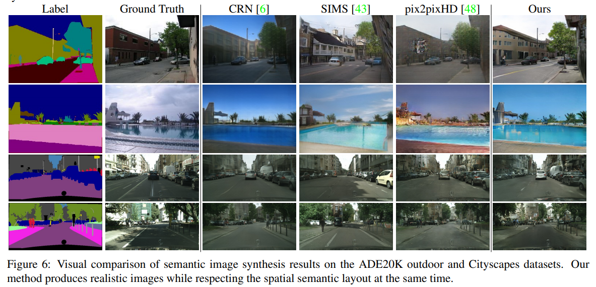
One can definitely observe the problem of mode averaging with Pix2PixHD output. We notice a smoothing/averaging effect seen in Pix2PixHD's output that seems to be smearing the low-level features of many objects.
For example, look at the building in the first row of images, or the water content in the second row of images. Pix2PixHD clearly struggles when there are large areas of a single object, and one can observe a smoothing effect which is causing a loss of detail. This is perhaps because of the issue we discussed earlier regarding the GAN struggling to create different information from a uniform swab of input values.
GauGAN fares much better here, perhaps because of its use of SPADE.
Apart from this, there are a couple of ways authors have tried to measure the performance of GauGAN quantitatively. We'll review them now.
mIoU Test
The first step of the mIoU test is to take the generated images and run a state of the art semantic segmentation algorithm on them. The result would be a semantic segmentation map for each generated image. Then, we compute the mIoU between the original semantic segmentation maps and the ones derived from generated images.
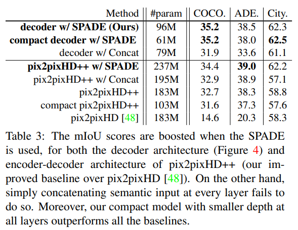
In order to check the importance of SPADE, the authors compare the result of Pix2PixHD with all the enhancements of GauGAN bar the SPADE generator. They call it the Pix2PixHD++. They also incorporate other architectures in this series of experiments, including a compact architecture with less layers and a Pix2PixHD-style encoder-decoder architecture, as opposed to the decoder-only architecture of GauGAN.
Frechet Inception Distance
Frechet Inception Distance (FID), in recent times, has turned out to be the favorite evaluation metric for researchers working on GANs. Again, it's not perfect, but it's certainly one of the best we've got. So, how does FID work?
We start by taking the real image $R$ and the fake image $F$ and putting them through an Inception v3 network. Then we take the 2048-dimensional pool layer of the network for both images and compute the distance between two extracted features. We do this for all of the semantic map-image pairs in our dataset. Then, using all of these vectors, we compute the FID using the following formula.

Where $\mu_r$ and $\mu_g$ are the means of the features of the real images and the generated images, respectively. $\sum_r$ and $\sum_g$ are the variance matrices. $T_r$ represents the Trace operator.
The idea here is to capture the statistics of an image (Inception v3 is taken as the statistic computation function) rather than the pixels of the two images. Since Inception v3 is color invariant (i.e. it will classify a car as a car, regardless of what color that car is), it's a superior choice to squared distance. Also, it ensures that factors like the time of day, color, and orientation don't really affect the score of a diverse image, since Inception is trained to be invariant to such differences.
This also helps ensure that the constraint does not force the network to overfit to the training data.
Limitations of the FID Score
However, since we are using an Inception v3 network as a judge for images, the results will theoretically be limited by how good the Inception v3 network is. Let's say it does not perform very well on images containing wild animals. If you're trying to generate images of zebras, then the scores might be a bit unpredictable because the algorithm might be sensitive to diverse images of zebras, and may produce randomly different feature vectors for two such images. Wild animals are just background for the network, we haven't specifically trained it to recognize two diverse images of zebras as belonging to a "zebra" class.
Now consider the following image from the Cityscapes Dataset.
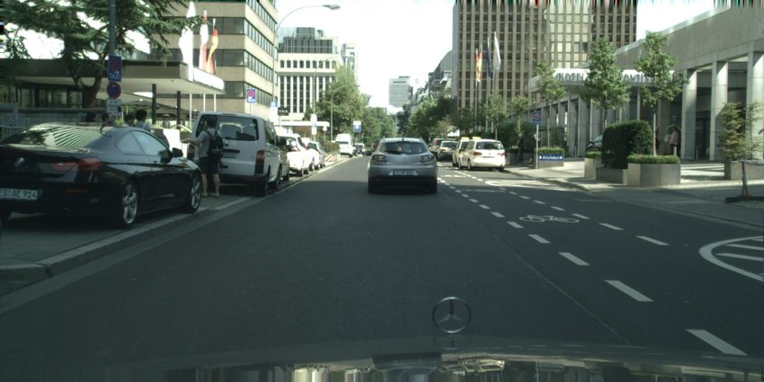
One of the most fundamental requirements for deep learning to work is to make sure that the data on which an algorithm is evaluated is the same or similar to the data on which it was trained. Consider, for example, an Inception v3 model trained on the ImageNet dataset.
If you have a look at the data from ImageNet, you will realize that the images are vastly different from the Cityscapes Dataset. First, the images are generally not very detailed; they typically contain only one object, which pretty much occupies all of the image. For example, take these images of a car.
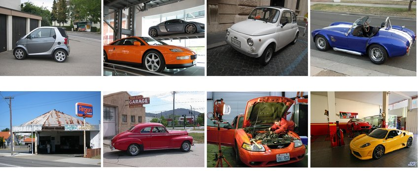
On the other hand, the images in Cityscapes are generally very detailed, containing many different objects.
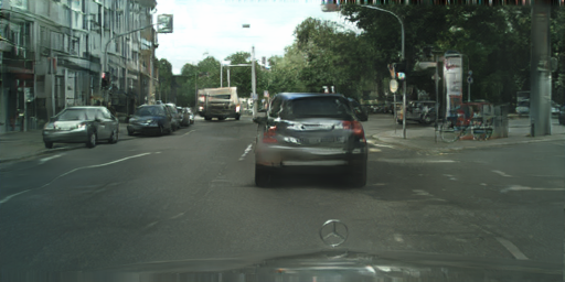
Sure, the layers of Inception v3 can capture these objects, but all objects will not be equally hard to synthesize. Areas like the sky and roads, which only constitute of rendering a texture, are much easier to render than let's say a car, which requires the algorithm to create structural details (like a bumper, backlights, and windows) as well.
Now, imagine a scenario where cars are rendered poorly while sky and roads are rendered fine. Also, the cars occupy a very small area of the image compared to the sky and the roads. The ill-rendered cars should keep the FID high, but they contribute too little to the feature vector as they occupy relatively little space in the image. On the other hand, the well-rendered sky/roads hardly increase the FID, and dominate the feature vector. This could lead to images with good background and bad foreground. Here is an example of that happening with data generated by using the official implementation on the Cityscapes Dataset.
Computing FID Score
In order to compute the FID score for your predictions we'll use the official implementation of FID. Note that I am not using the official FID score repo, which is something that you should use in case you are reporting your results. The reason why I don't use it is because it's written for Tensorflow, and the recent updates in TensorFlow–especially with version 2.0–have broken a lot of code. So, better to use something more stable. For the curious, the official repo can be found here.
We first begin by cloning the repo.
git clone https://github.com/mseitzer/pytorch-fid
cd pytorch-fid
Now, FID will be used to compare our original data and the generated data. Before we can do that, make sure that you are comparing images of the same size. For example, your training data might have size 2048 x 512, while GauGAN is configured to produce images with the dimensions 1024 x 512. Such disparity in size may lead to a larger FID than it truly is.
Once that's done, the job is pretty easy. You can compute the FID with the following piece of code:
python fid_score.py /path/to/images /path/to/other_images --batch-size b
Choose the batch size so that the total number of your test images are a multiple of your batch size b . If that's not possible, make sure that the remainder is minimized. For example, for 71 test images, you may choose a batch size of 7 (since 71 is a prime number).
One might also consider resizing the images generated by GANs to the size of the original image. However, it would not be a fair metric for the GAN since it has been supervised (during its training) with images of lower dimensionality only.
Summing Up GauGAN's Performance
Here is a table from the original GauGAN paper that sums up how GauGAN performs against its adversaries.
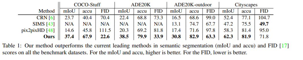
That being said, you could run into reproducibility issues. The failure to reproduce results is a big issue for the deep learning community, and Nvidia's latest offerings are not immune to it.
Conclusion
That concludes Part 3 of our series. In the fourth and final part we take a look at common troubleshooting tips, the costs of GauGAN from a business perspective, and why you might want to skip GauGAN and wait for the technology to mature. Till then, here are some links you can follow to read more about the topics mentioned in the article.
Understanding GauGAN Series
- Part 1: Unraveling Nvidia's Landscape Painting GANs
- Part 2: Training on Custom Datasets
- Part 3: Model Evaluation Techniques
- Part 4: Debugging Training & Deciding If GauGAN Is Right For You