Introduction to Naive Bayes: A Probability-Based Classification Algorithm

Imagine this: an electricity operator would like to supply specific units of electric current to various factory divisions based on their past trends of power consumption. To simplify the process, she/he plans to categorize the factory divisions into three groups–low, medium, and high-power consumers–based on which he knows how much electricity to supply. Problems of this type usually fall under predictive classification modeling, or are simply known as classification-type problems. Naive Bayes is one of the simplest Machine Learning algorithms that has always been a favorite for classifying data.

Naive Bayes is based on Bayes Theorem, which was proposed by Reverend Thomas Bayes back in the 1760's. Its popularity has skyrocketed in the last decade and the algorithm is widely being used to tackle problems across academia, government, and business. A Naive Bayes classifier is an amalgamation of a number of desirable qualities in practical machine learning. We'll shed light on the intuitions behind this further on. Let’s get started by first understanding the working of a Naive Bayes algorithm, and then implementing it in Python using the scikit-learn library.

In this article we'll learn about the following topics:

• Introduction to Naive Bayes Algorithm
• Conditional Probability and Bayes Theorem
• Working of Naive Bayes Algorithm
• Applications of Naive Bayes
• Implementing Naive Bayes with Scikit-Learn
• Pros and Cons
• Summary

Introduction to Naive Bayes Algorithm

Naive Bayes falls under the umbrella of supervised machine learning algorithms that are primarily used for classification. In this context, "supervised" tells us that the algorithm is trained with both input features and categorical outputs (i.e., the data includes the correct desired output for each point, which the algorithm should predict).

But why is the algorithm called "naive"? This is because the classifier assumes that the input features that go into the model are independent of each other. Hence, changing one input feature won’t affect any of the others. It's therefore naive in the sense that this assumption may or may not be true, and it most probably isn't.

We’ll discuss the naiveness of this algorithm in detail in the Working of Naive Bayes Algorithm section. Before that, let’s briefly look at why this algorithm is simple, yet powerful, and easy to implement. One of the significant advantages of Naive Bayes is that it uses a probabilistic approach; all the computations are done on the fly in real time, and outputs are generated instantaneously. When handling large amounts of data, this gives Naive Bayes an upper hand over traditional classification algorithms like SVMs and Ensemble techniques.

Let’s get started by getting a hang of the theory essential to understanding Naive Bayes.

Probability, Conditional Probability, and Bayes Theorem

Probability is the foundation upon which Naive Bayes has been built. Let’s get down to the nitty-gritty of what probability is all about.

What Is Probability?

Probability is one of the crucial branches of mathematics that helps us predict how likely an event X is to happen considering the total of potential outcomes. To explain this in a more precise way, consider a case of making a prediction on whether you would go to college on a specific day. Here there are two possible outcomes: attend or skip. Thus, the probability of you attending or skipping college is ½. Mathematically, probability can be represented by the following equation:

Probability of an Event = Number of Favorable Events / Total Number of Outcomes

0 <= Probability of an Event <= 1

The "favorable events" denote the event(s) for which you want the probability of their occurring. Probability always lies in the range of 0 to 1, with 0 meaning there’s no possibility of that event happening, and 1 meaning there’s a 100% possibility it will happen.

Conditional Probability is a subset of Probability, which restricts the idea of probability to create a dependency on a specific event; let’s understand it in the next section.

Conditional Probability

Conditional probability is computed for two or more events. Take two events, A and B. The conditional probability of event B is defined as the probability that event B will occur given the knowledge that event A has already happened. It is represented as P(B|A), and mathematically by the formula:

P(B|A) = P(A and B)/P(A)

Let’s look at an example to understand the concept clearly.

Consider you have two baskets, Basket A and Basket B, which are filled with both Apples and Mangoes. The composition details are shown below:

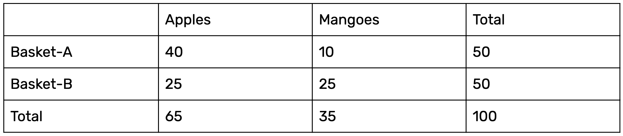
To find the conditional probability of a randomly selected fruit being an Apple taken from Basket-B, we use the above formula as follows:

P(Apple/Basket-B) = P(Apple and Basket-B)/ P(Basket-B)
                  = 25/50

This probability reflects first choosing Basket-B and then picking an apple from it.

In the next section we'll look at Bayes theorem, which follows in the footsteps of Conditional probability.

Bayes Rule

Bayes Rule revolves around the concept of deriving a hypothesis (H) from the given evidence (E). It relates two notions: the probability of the hypothesis before getting the evidence, P(H), and the probability of the hypothesis after getting the evidence, P(H|E).  In general, it’s given by the following equation:

P(H|E) = (P(E|H) * P(H)) / P(E)

Which tells us:

• How often H happens given that E happens, written as P(H|E)

When we know:

• How often E happens given that H happens, written as P(E|H)
• How likely A is on its own, written as P(H)
• How likely B is on its own, written as P(E)

The Bayes Rule is a way of going from P(E|H) to finding P(H|E). In simple terms, it provides a way to calculate the probability of a hypothesis given the evidence.

Bayes Rule from a Machine Learning Perspective

We usually have training data to teach our model, and validation data to evaluate the model and make new predictions. Let’s call our input features as evidence, and labels as outcomes in the training data. Using conditional probability, we calculate the probability of the evidence given the outcomes, denoted as P(Evidence|Outcome). Our goal now is to find the probability of an outcome with respect to the evidence, denoted as P(Outcome|Evidence).  Let’s define Bayes Rule for both, P(Evidence|Outcome) and P(Outcome|Evidence).

Consider X to denote Evidence and Y to denote Outcome.

P(Evidence|Outcome) is thus P(X|Y), and is represented as follows:

P(X|Y) = (P(Y|X) * P(X)) / P(Y) (To be estimated from the training data.)

P(Outcome|Evidence) is P(Y|X), and is represented as follows:

P(Y|X) = (P(X|Y) * P(Y)) / P(X) (To be predicted from the test data.)

If the problem at hand has two outcomes, then we calculate the probability of each outcome and say the highest one wins. But what if we have multiple input features? This is when Naive Bayes comes into the picture; let’s discuss this algorithm in the next section.

Working of the Naive Bayes Algorithm

The Bayes Rule provides the formula to compute the probability of output (Y) given the input (X). In real-world problems, unlike the hypothetical assumption of having a single input feature, we have multiple X variables. When we can assume the features are independent of each other, we extend the Bayes Rule to what is called Naive Bayes.

Consider a case where there are multiple inputs (X1, X2, X3,... Xn). We predict the outcome (Y) using the Naive Bayes equation as follows:

P(Y=k | X1...Xn) =  ( P(X1 | Y=k) * P(X2 | Y=k) * P(X3 | Y=k) * ....* P(Xn | Y=k) ) * P(Y=k) / P(X1)*P(X2)*P(X3)*P(Xn)

In the above formula:

• P(Y=k | X1...Xn) is called the Posterior Probability, which is the probability of an outcome given the evidence.
• P(X1 | Y=k) * P(X2 | Y=k) * ... P(Xn | Y=k) is the probability of the likelihood of evidence.
• P(Y=k) is the Prior Probability.
• P(X1)*P(X2)*P(Xn) is the probability of the evidence.

A clear-cut example should give you insight into how the above equation is put into practice. Let’s consider a simple dataset comprised of 10 data samples:

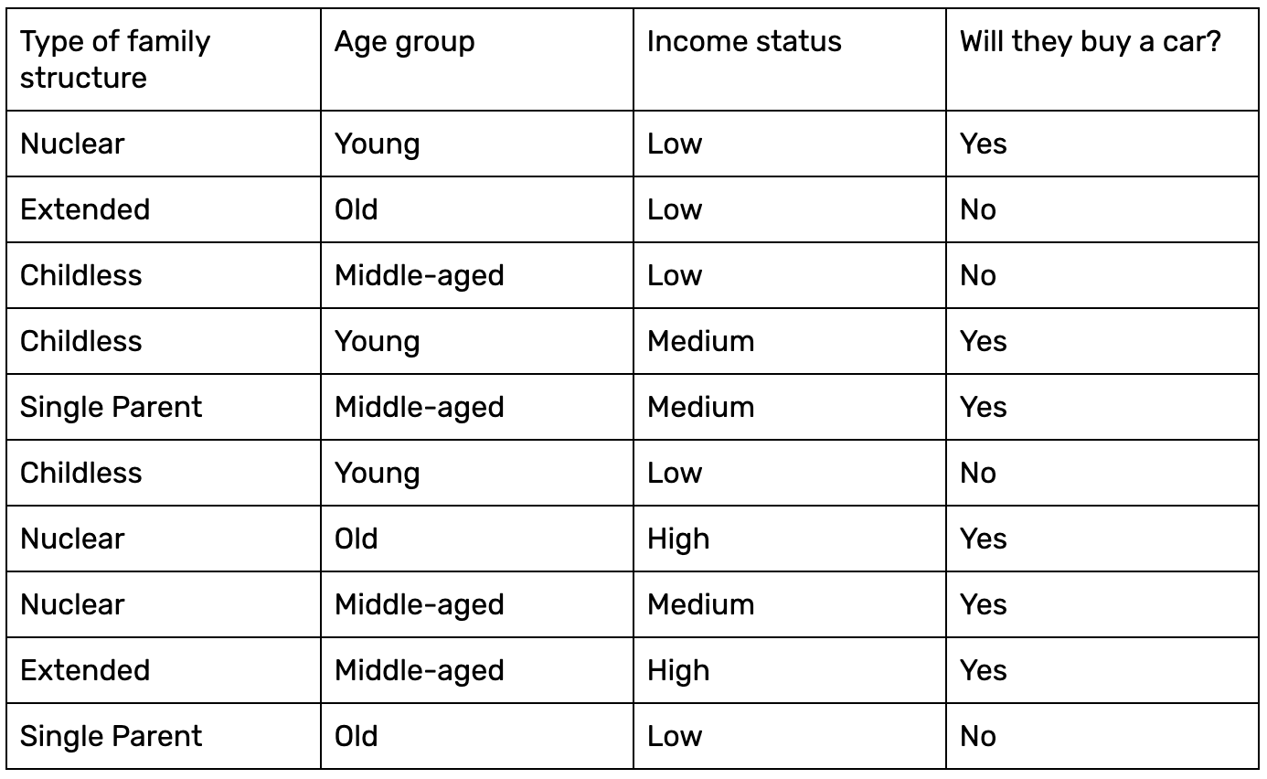
Given three inputs–for example, Single Parent, Young, and Low–we want to compute the probability of these people buying a car. Let’s use Naive Bayes.

Firstly, let’s compute the probability of the output labels (P(Y)) given the data.

P(No) = 4/10

P(Yes) = 6/10

Now let’s calculate the probability of the likelihood of the evidence. Given the inputs Childless, Young, and Low, we'll calculate the probability with respect to both class labels as follows:

P(Single Parent|Yes) = 1/6
P(Single Parent|No) = 1/4
P(Young|Yes) = 2/6
P(Young|No) = 1/4
P(Low|Yes) = 1/6
P(Low|No) = 4/4

Since P(X1) * P(X2) * ... * P(Xn) remains the same when calculating the probability for both Yes and No output labels, we can eliminate that value.

Thus, the posterior probability is computed as follows (note that X is the test data):

P(Yes|X) = P(Single Parent|Yes) * P(Young|Yes) * P(Low|Yes) = 1/6 * 2/6 * 1/6 = 0.0063

P(No|X) = P(Single Parent|No) * P(Young|No) * P(Low|No) = 1/4 * 1/4 * 4/4 = 0.0625

The final probabilities are:

P(Yes|X) = 0.0063/(0.0063 + 0.0625) = 0.09
P(No|X) = 0.0625/(0.0063 + 0.0625) = 0.91

Thus, the results clearly show that the car probably will not be purchased.

We previously mentioned that the "naiveness" of the algorithm is that it assumes each feature is independent of the others. We calculated the probabilities with respect to the output label with this assumption, so that each feature has an equal contribution and is independent of all the other features. This indeed is the naive assumption.

Applications

Below are a few use cases that employ Naive Bayes:

• Real-time prediction: Naive Bayes is an eager learning classifier and is quite fast in its execution. Thus, it could be used for making predictions in real-time.
• Multi-class prediction: The Naive Bayes algorithm is also well-known for multi-class prediction, or classifying instances into one of several different classes.
• Text classification/spam filtering/sentiment analysis: When used to classify text, a Naive Bayes classifier often achieves a higher success rate than other algorithms due to its ability to perform well on multi-class problems while assuming independence. As a result, it is widely used in spam filtering (identifying spam email) and sentiment analysis (e.g. in social media, to identify positive and negative customer sentiments).
• Recommendation Systems: A Naive Bayes Classifier can be used together with Collaborative Filtering to build a Recommendation System which could filter through new information and predict whether a user would like a given resource or not.

Implementation of Naive Bayes with Scikit-Learn

Now we'll use the scikit-learn library to build a Naive Bayes classifier.

Step 1: Let's use a toy dataset with just three columns in it: weather, temperature, and play. The first two are features (weather and temperature) and the third is the target label (whether or not children go out to play).

# Assigning features and label variables
weather = ['Sunny','Sunny','Overcast','Rainy','Rainy','Rainy','Overcast','Sunny','Sunny','Rainy','Sunny','Overcast','Overcast','Rainy']
temp = ['Hot','Hot','Hot','Mild','Cool','Cool','Cool','Mild','Cool','Mild','Mild','Mild','Hot','Mild']
play = ['No','No','Yes','Yes','Yes','No','Yes','No','Yes','Yes','Yes','Yes','Yes','No']

Step 2: We'll need to convert string labels (as seen in the toy dataset) into numbers. For example, we could map 'Overcast', 'Rainy', and 'Sunny' to 0, 1, and 2 respectively. This is known as label encoding. Scikit-learn provides the LabelEncoder library for encoding data items to a value that lies between 0 and one less than the number of discrete classes (in our case, that’s 2 for both weather and temp, and 1 for play). For now, let’s encode the weather column as follows:

# Import LabelEncoder
from sklearn import preprocessing

# Creating labelEncoder
le = preprocessing.LabelEncoder()

# Converting string labels into numbers.
weather_encoded=le.fit_transform(weather)
print(weather_encoded)

Output: [2 2 0 1 1 1 0 2 2 1 2 0 0 1]

Step 3: Similarly, we can also encode the temp and play columns.

# Converting string labels into numbers
temp_encoded = le.fit_transform(temp)
label = le.fit_transform(play)
print("Temp:",temp_encoded)
print("Play:",label)

Output:
Temp: [1 1 1 2 0 0 0 2 0 2 2 2 1 2]
Play: [0 0 1 1 1 0 1 0 1 1 1 1 1 0]

Step 4: Let’s now merge the weather and temp attributes element-wise, i.e. merge the 1D feature arrays into a 2D array. This will make our task easier for building the sklearn model. We use the vstack function from the NumPy library to accomplish this.

Output:
array([[2, 1],
       [2, 1],
       [0, 1],
       [1, 2],
       [1, 0],
       [1, 0],
       [0, 0],
       [2, 2],
       [2, 0],
       [1, 2],
       [2, 2],
       [0, 2],
       [0, 1],
       [1, 2]], dtype=int64)

Step 5: Let’s generate our Naive Bayes model using the following steps:

1. Create a Naive Bayes classifier using GaussianNB by importing it from sklearn.naive_bayes.
2. Fit the dataset on classifier using model.fit.
3. Make a prediction using model.predict.

# Import Gaussian Naive Bayes model
from sklearn.naive_bayes import GaussianNB

# Create a Gaussian Classifier
model = GaussianNB()

# Train the model using the training sets
model.fit(com,label)

# Predict Output
predicted= model.predict([[0,2]]) # 0:Overcast, 2:Mild
print ("Predicted Value:", predicted)

Output: [1]

‘1’ here is the target value, or ‘yes’. GaussianNB is the Gaussian Naive Bayes algorithm wherein the likelihood of the features is assumed to be Gaussian.

Advantages of Naive Bayes

• Naive Bayes is easy to grasp and works quickly to predict class labels. It also performs well on multi-class prediction.
• When the assumption of independence holds, a Naive Bayes classifier performs better compared to other models like logistic regression, and you would also need less training data.
• It performs well when the input values are categorical rather than numeric. In the case of numerics, a normal distribution is assumed to compute the probabilities (a bell curve, which is a strong assumption).

Disadvantages of Naive Bayes

• If a categorical variable has a category in the test data set, which is not observed by the model in the training data, it will assign a 0 (zero) probability and not be able to make a prediction. This is often referred to as “Zero Frequency”. To solve this problem, we can use the smoothing technique. One of the simplest smoothing techniques is called Laplace estimation.
• The other limitation of Naive Bayes is the assumption of independence among the features. In real life, it is almost impossible that we get a set of features that are completely independent.

Summary

Though Naive Bayes has a handful of limitations, it’s still a go-to algorithm to classify data, primarily due to its simplicity. It has worked particularly well for document classification and spam filtering. For a more hands-on understanding of Naive Bayes, I recommend you try using what we implemented on various other datasets to gain a deeper insight into how Naive Bayes analyzes and classifies the data.

References

1. https://www.analyticsvidhya.com/blog/2017/09/naive-bayes-explained/
2. https://machinelearningmastery.com/naive-bayes-for-machine-learning/
3. https://www.datacamp.com/community/tutorials/naive-bayes-scikit-learn
4. https://becominghuman.ai/naive-bayes-theorem-d8854a41ea08
5. https://brilliant.org/wiki/bayes-theorem/