Object Localization using PyTorch, Part 1

The Deep Learning domain got its attention with the popularity of Image classification models, and the rest is history. Today, we are generating future tech just from a single image input. GAN models generate an image, image segmentation models mark regions accurately, and object detection models detect everything going on, like identifying the people in a busy street just from an ordinary CCTV camera. These achievements have truly paved the way for further research, and also acceptance of basic modeling practices into serious domains like the Medical field along with the arrival of Explainable AI. Image localization is an interesting application for me as it falls right between Image Classification and Object Detection. Whenever one has to get bounding boxes over a detected category for a project, people frequently jump to object detection and YOLO, which are great, but really overkill in my opinion if you are just doing classification and locating that single class. Let us dive deep into Image Localization: the concept, implementation in PyTorch, and possibilities.

Image Classification

Image classification is one of the basic deep learning problems that is solved using convolutional neural networks, and the architectures built on them, ResNet, SqueezeNet, etc., improved the performance of such models to a great extent over time. Depending on the project, it is not always the requirement to build a huge model over the size of 250MB that gives 95+% validation accuracy. Sometimes while developing, like for mobile platforms like Lens Studio, it is important that you get a smaller model in terms of size and computation with justifiable accuracy that has very small inference time. In this smaller model space, we have models like MobileNet, SqueezeNet, etc.

This diversity in architectures and use cases led to improvements in classification and leading to object localization.  The idea that a model can not just classify an image into x or y, but have the ability to locate x or y in the image with a strong bounding box, exponentially increases the use cases that can be built around it. The approach towards localization is pretty similar to image classification, so it might be difficult to jump in if you are not familiar with CNNs. Let us explore them a bit before going further in the localization domain.

Convolutional Neural Nets

If you are new to neural networks, kindly give this a read.

Assuming you understand how deep learning models work on a basic fully connected layer model, they become computationally heavy as parameters keep increasing and as fully connected layers of huge size get added on.

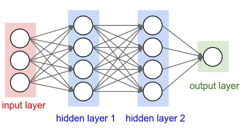
Here if you look at the image above, focusing on the red and the first blue layer, the computation between them will take (not accurately, just for illustration) 3*4 operations. Now, this is pretty lightweight for even a CPU. But when we are dealing with images, let us take a typical 64X64 size image. The images are of size 64x64, having 3 channels each. That’s a total of 12,288 pixels across RGB channels for each of the images. Now, this sounds huge, but it just gets bigger computationally when you think of dealing with images the same way as the fully connected layer above. When you multiply every neuron out of the 12288 one with the others on the next layer, which is really expensive from a computational standpoint, cost explodes upward.

To remedy this, we can employ CNNs: which do the tasks in a much more computationally lighter manner to many heavier model architectures while giving better accuracy. In Convolutional Neural Networks, we do computation over tensors with the kernel over channels, and keep on reducing the size of the tensor, while increasing the number of channels where each channel contributes to learning something unique, until we then finally flatten the stack of channels to a fully connected layer like is shown below. This is a brief explanation of CNNs, one must dive deep into the architecture to master every aspect of it.

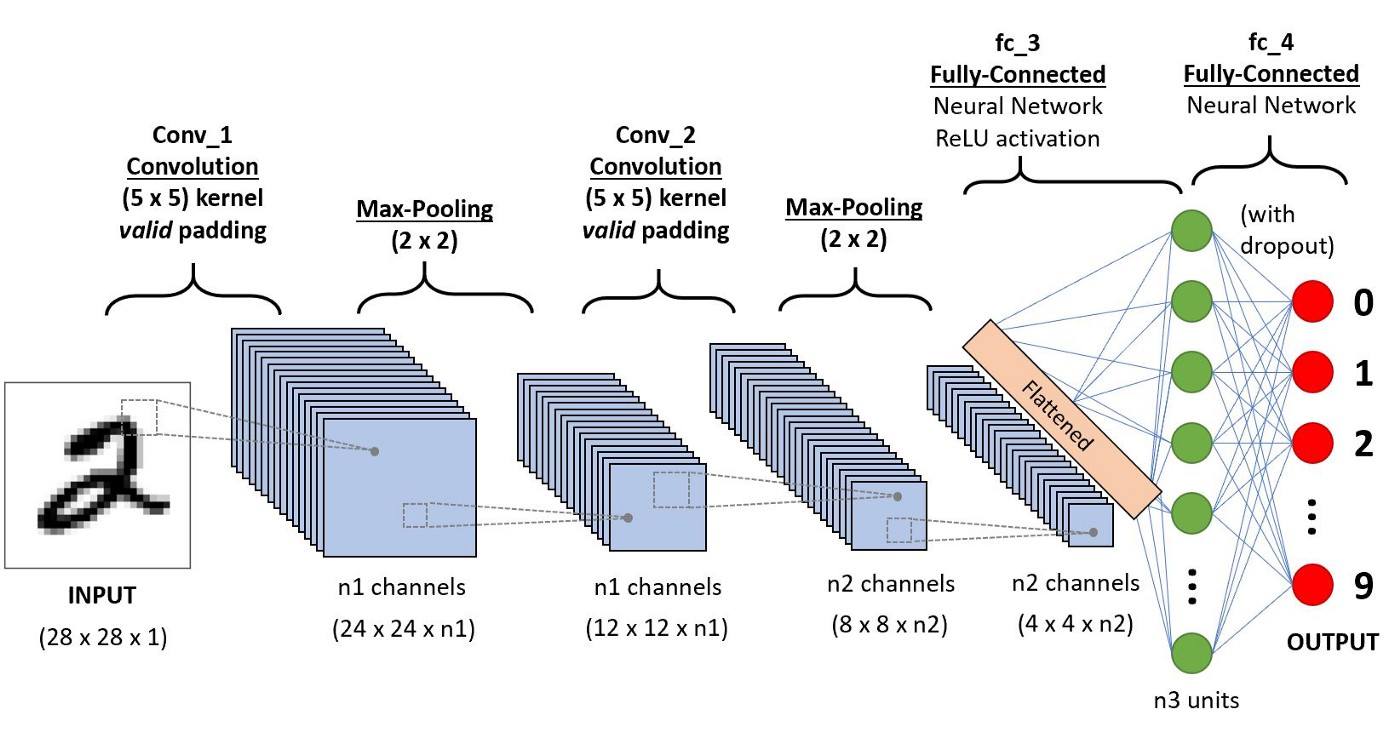
Before going to object localization, focus on the red dot layer above. That serves as the last layer of the image classification problem and the result is the index of the neuron with maximum value. That is the predicted class index. In object localization, we will have not just one output, but 2 different outputs, one being the class and the other being a regression output having 4 values of the bounding box coordinates.  

Object Localization

The fascinating part about localization is the simplicity it has compared to object detection models. Definitely, object detection models deal with a much bigger problem, and have to run classification for all the regions suggested by the initial region selection layer in certain architectures. Still, the idea that we can predict the coordinates like a regression problem is interesting. So our general architecture, which is similar to an image classification model, will have additionally 1 regression output (with 4 coordinates) training in parallel towards getting the coordinates.

Dataset for Localization

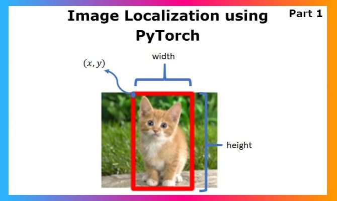
For object localization, we will need not just the image and label, but also the coordinates of the bounding box containing the object. We must use image annotation/object tagging tools for preparing such a dataset, and XML is a popular file format used to store coordinate values of each image.

One of the more popular object tagging tools is Microsoft's open source object tagging tool, VOTT. It is lightweight and simple which makes it perfect for localization problems. Here is the link to the project and the documentation.

It is not compulsory that you store the data as XML, you can choose any file type which you are comfortable handling for data reading, but XMLs work like a charm. Our inputs will be the image, its label, and four values corresponding to the coordinates we are tagging. For this project, I extracted a part of the popular Dogs vs. Cats Dataset, and created bounding boxes using VOTT and generated XML files. We shall discuss in detail how we can read those XML files to obtain the input coordinates for the corresponding image with the power of python and some libraries.

PyTorch Implementation

As usual, we are starting off with importing libraries including pandas, CSV, and XML which will help us work on the inputs.

import numpy as np

from sklearn.model_selection import train_test_split

import matplotlib.pyplot as plt
import cv2
import random
import os

from PIL import Image

import pandas as pd
from xml.dom import minidom
import csv

You can download the dataset used to demonstrate this object localization implementation from here. When implementing for your personal projects, alter the dataset and populate it with more images and annotations for reliable model performance. As I had to create bounding boxes for the sake of the demo, I have kept the samples to a minimum.

First, we shall unzip the dataset to get started. The Dataset link is given above.

!unzip localization_dataset.zip

Let us analyze the XML file before reading and processing the inputs. Understanding the structure will help you understand how to read a new XML when you encounter it.

<annotation verified="yes">
    <folder>Annotation</folder>
    <filename>cat.0.jpg</filename>
    <path>Cat-PascalVOC-export/Annotations/cat.0.jpg</path>
    <source>
        <database>Unknown</database>
    </source>
    <size>
        <width>256</width>
        <height>256</height>
        <depth>3</depth>
    </size>
    <segmented>0</segmented>
    <object>
    <name>cat</name>
    <pose>Unspecified</pose>
    <truncated>0</truncated>
    <difficult>0</difficult>
    <bndbox>
        <xmin>55.35820533192091</xmin>
        <ymin>10.992090947210452</ymin>
        <xmax>197.38757944915255</xmax>
        <ymax>171.24521098163842</ymax>
    </bndbox>
</object>
</annotation>

Next, let's jump into reading and processing the images and annotations. We shall use  XML minidom to read xml files.

def extract_xml_contents(annot_directory, image_dir):
        
        file = minidom.parse(annot_directory)

        # Get the height and width for our image
        height, width = cv2.imread(image_dir).shape[:2]

        # Get the bounding box co-ordinates 
        xmin = file.getElementsByTagName('xmin')
        x1 = float(xmin[0].firstChild.data)

        ymin = file.getElementsByTagName('ymin')
        y1 = float(ymin[0].firstChild.data)

        xmax = file.getElementsByTagName('xmax')
        x2 = float(xmax[0].firstChild.data)

        ymax = file.getElementsByTagName('ymax')
        y2 = float(ymax[0].firstChild.data)

        class_name = file.getElementsByTagName('name')

        if class_name[0].firstChild.data == "cat":
          class_num = 0
        else:
          class_num = 1

        files = file.getElementsByTagName('filename')
        filename = files[0].firstChild.data

        # Return the extracted attributes
        return filename,  width, height, class_num, x1,y1,x2,y2

Let us create a num_to_labels dictionary for retrieving the labels from predictions.

num_to_labels= {0:'cat',1:'dog'}

Once we get all this data, we can store this as a CSV, so that we don't have to read the XML files for each run of training. We shall use a Pandas data frame for storing the data which we shall later save as a CSV.

# Function to convert XML files to CSV
def xml_to_csv():

  # List containing all our attributes regarding each image
  xml_list = []

  # We loop our each class and its labels one by one to preprocess and augment 
  image_dir = 'dataset/images'
  annot_dir = 'dataset/annot'

  # Get each file in the image and annotation directory
  mat_files = os.listdir(annot_dir)
  img_files = os.listdir(image_dir)

  # Loop over each of the image and its label
  for mat, image_file in zip(mat_files, img_files):
      
      # Full mat path
      mat_path = os.path.join(annot_dir, mat)

      # Full path Image
      img_path = os.path.join(image_dir, image_file)

      # Get Attributes for each image 
      value = extract_xml_contents(mat_path, img_path)

      # Append the attributes to the mat_list
      xml_list.append(value)

  # Columns for Pandas DataFrame
  column_name = ['filename', 'width', 'height', 'class_num', 'xmin', 'ymin', 
                 'xmax', 'ymax']

  # Create the DataFrame from mat_list
  xml_df = pd.DataFrame(xml_list, columns=column_name)

  # Return the dataframe
  return xml_df

# The Classes we will use for our training
classes_list = sorted(['cat',  'dog'])

# Run the function to convert all the xml files to a Pandas DataFrame
labels_df = xml_to_csv()

# Saving the Pandas DataFrame as CSV File
labels_df.to_csv(('dataset.csv'), index=None)

Now that we got the data in the CSV, let us load the corresponding images and labels for building data loaders. We will be pre-processing images, including normalizing the pixels. One thing to note here is how we store the coordinates. We are storing the value as a 0 to 1 range value by dividing it with image size (256 here) so that the model output can be scaled to any image later (we will see this in the visualization part).  

def preprocess_dataset():
  # Lists that will contain the whole dataset
  labels = []
  boxes = []
  img_list = []

  h = 256
  w = 256
  image_dir = 'dataset/images'

  with open('dataset.csv') as csvfile:
      rows = csv.reader(csvfile)
      columns = next(iter(rows))
      for row in rows:
        labels.append(int(row[3]))
        #Scaling Coordinates to the range of [0,1] by dividing the coordinate with image size, 256 here.
        arr = [float(row[4])/256,  
               float(row[5])/256,
               float(row[6])/256,
               float(row[7])/256]
        boxes.append(arr)
        img_path = row[0]
        # Read the image
        img  = cv2.imread(os.path.join(image_dir,img_path))

        # Resize all images to a fix size
        image = cv2.resize(img, (256, 256))

        # # Convert the image from BGR to RGB as NasNetMobile was trained on RGB images
        image = cv2.cvtColor(image, cv2.COLOR_BGR2RGB)

        # Normalize the image by dividing it by 255.0 
        image = image.astype("float") / 255.0

        # Append it to the list of images
        img_list.append(image)

  return labels, boxes, img_list

Now that function is ready, let us call it and load the data for inputs. As a final step of Data Preprocessing, we shall shuffle the data.

# All images will resized to 300, 300 
image_size = 256

# Get Augmented images and bounding boxes
labels, boxes, img_list = preprocess_dataset()

# Now we need to shuffle the data, so zip all lists and shuffle
combined_list = list(zip(img_list, boxes, labels))
random.shuffle(combined_list)

# Extract back the contents of each list
img_list, boxes, labels = zip(*combined_list)

So far we have completed the data preprocessing involving reading the data annotations from XML files and now we are ready to proceed with building custom Data Loaders in PyTorch and Model Architecture design. The Implementation will continue in the next part of this article where we shall discuss the above-mentioned approaches in detail to complete the implementation. Thanks for reading :)