In Part 1 of this series we looked at time series analysis. We learned about the different properties of a time series, autocorrelation, partial autocorrelation, stationarity, tests for stationarity, and seasonality.
In this part of the series, we will see how we can make models that take a time series and predict how the series will move in the future. Specifically, in this tutorial, we will look at autoregressive models and exponential smoothing methods. In the final part of the series, we will look at machine learning and deep learning algorithms like linear regression and LSTMs.
You can also follow along with the code in this article (and run it for free) from a Gradient Community Notebook on the ML Showcase.
Bring this project to life
We will be using the same data we used in the previous article (i.e. the weather data from Jena, Germany) for our experiments. You can download it using the following command.
wget https://storage.googleapis.com/tensorflow/tf-keras-datasets/jena_climate_2009_2016.csv.zipUnzip the file and you'll find CSV data that you can read using Pandas. The dataset has several different weather parameters recorded. For this tutorial, we'll be using Temperature in Celsius. The data is recorded regularly over 24 hour periods at 10 minute intervals. We will be using hourly data for our predictive models.
import pandas as pd

df = pd.read_csv('jena_climate_2009_2016.csv')

time = pd.to_datetime(df.pop('Date Time'), format='%d.%m.%Y %H:%M:%S')
series = df['T (degC)'][5::6]
series.index = time[5::6]
There are different methods applied for time series forecasting, depending on the trends we discussed in the previous article. If a time series is stationary, autoregressive models can come in handy. If a series is not stationary, smoothing methods might work well. Seasonality can be handled in both autoregressive models as well as smoothing methods. We can also use classical machine learning algorithms like linear regression, random forest regression, etc., as well as deep learning architectures based on LSTMs.
If you haven't read the first article in this series, I would suggest you read through it before diving into this one.
Autoregressive Models
In multiple linear regression, we predict a value based on the value of other variables. The expression for the model assumes a linear relationship between the output variable and the predictor variables.
In autoregressive models, we assume a linear relationship between the value of a variable at time $t$ and the value of the same variable in the past, that is time $t-1, t-2, ..., t-p, ..., 2, 1, 0$.
$$ y_{t} = c + \beta_{1}y_{t -1} + \beta_{2}y_{t -2} + ... + \beta_{p}y_{t -p} + \epsilon_{t}$$
Here p is the lag order of the autoregressive model.
For an AR(1) model,
- When $\beta_1 = 0$, it signifies random data
- When $\beta_1 = 1$ and $c = 0$, it signifies a random walk
- When $\beta_1 = 1$ and $c \neq 0$, it signifies a random walk with a drift
We usually restrict autoregressive models for stationary time series, which means that for an AR(1) model $-1 < \beta_1 < 1$.
Another way of representing a time series is by considering a pure Moving Average (MA) model, where the value of our variable depends on the residual errors of the series in the past.
$$ y_{t} = m + \epsilon_{t} + \phi_{1}\epsilon_{t -1} + \phi_{2}\epsilon_{t -2} + ... + \phi_{q}\epsilon_{t -q} $$
As we learned in the previous article, if a time series is not stationary, there are multiple ways of making it stationary. The most commonly used method is differencing.
ARIMA models take into account all the three mechanisms mentioned above and represent a time series as shown below.
$$ y_{t} = \alpha + \beta_{1}y_{t -1} + \beta_{2}y_{t -2} + ... + \beta_{p}y_{t -p} + \epsilon_{t} + \phi_{1}\epsilon_{t -1} + \phi_{2}\epsilon_{t -2} + ... + \phi_{q}\epsilon_{t -q}$$
(Where the series is assumed to be stationary.)
The stationarizing mechanism is implemented before the model is fitted on the series.
The order of differencing can be found by using different tests for stationarity and looking at PACF plots. You can refer to the first part of the series to understand the tests and their implementations.
The MA order is based on the ACF plots for differenced series. The order is decided depending on the order of differencing required to remove any autocorrelation in the time series.
You can implement this as follows, where $p$ is the lag order, $q$ is the MA order, and $d$ is the differencing order.
from matplotlib import pyplot as plt
from sklearn.metrics import mean_squared_error
from statsmodels.tsa.arima_model import ARIMA


def ARIMA_model(df, p=1, q=1, d=1):
    model = ARIMA(df, order=(p, d, q))
    results_ARIMA = model.fit(disp=-1)
    rmse = np.sqrt(mean_squared_error(df[1:], results_ARIMA.fittedvalues))
    return results_ARIMA, rmse
This will not be enough for our time series, because apart from being non-stationary, the time series we have also has seasonal trends. We will need a SARIMA model.
The equation for the SARIMA model becomes (assuming a seasonal lag of 12):
$$ y_{t} = \gamma + \beta_{1}y_{t -1} + \beta_{2}y_{t -2} + ... + \beta_{p}y_{t -p} + \\ \epsilon_{t} + \phi_{1}\epsilon_{t -1} + \phi_{2}\epsilon_{t -2} + ... + \phi_{q}\epsilon_{t -q} + \\ \Beta_{1}y_{t - 12} + \Beta_{2}y_{t - 13} + ... + \Beta_{q}y_{t - 12 - q} + \\ \epsilon_{t - 12} + \Phi_{1}\epsilon_{t -13} + \Phi_{2}\epsilon_{t - 14} + ... + \Phi_{q}\epsilon_{t - 12 - q}$$
This is a linear equation and the coefficients can be found using regression algorithms.
Sometimes a time series can be over- or under-differenced because the ACF and PACF plots can be a little tricky to infer from. Lucky for us, there is a tool we can use to automate the hyperparameter selection of ARIMA parameters as well as the sesonality. You can install pmdarima using pip.
pip install pmdarimapmdarima uses grid search to search through all the values of ARIMA parameters, and picks the model with the lowest AIC value. It also automatically calculates the difference value using the test you select for stationarity.
For our time series, though, the frequency is 1 cycle per 365 days (which is 1 cycle per 8544 data points). This can get a little too heavy for your computer to handle. Even after I reduced the data from hourly to daily, I found the modeling script getting killed. The only thing left for me to do was to convert the data to monthly and then run the model.
import pandas as pd
import matplotlib.pyplot as plt
import pmdarima as pm
import pickle
df = pd.read_csv('jena_climate_2009_2016.csv')
series = df['T (degC)'][4391::4392]
time = pd.to_datetime(df.pop('Date Time'), format='%d.%m.%Y %H:%M:%S')[4391::4392]
series.index = time
train = series[:-int(len(series)/10)]
test = series[-int(len(series)/10):]
model = pm.auto_arima(train.values,
start_p=1, # lag order starting value
start_q=1, # moving average order starting value
test='adf', #ADF test to decide the differencing order
max_p=3, # maximum lag order
max_q=3, # maximum moving average order
m=12, # seasonal frequency
d=None, # None so that the algorithm can chose the differencing order depending on the test
seasonal=True,
start_P=0,
D=1, # enforcing the seasonal frequencing with a positive seasonal difference value
trace=True,
suppress_warnings=True,
stepwise=True)
print(model.summary())
# save the model
with open('seasonal_o.pkl', 'wb') as f:
pickle.dump(model, f)
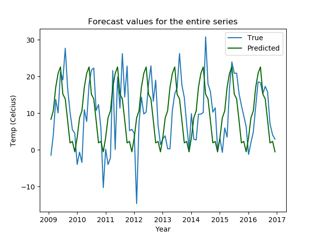
# predictions for the entire series
all_vals = model.predict(n_periods=len(series), return_conf_int=False)
all_vals = pd.Series(all_vals, index=series.index)
plt.plot(series)
plt.plot(all_vals, color='darkgreen')
plt.title('Forecast values for the entire series')
plt.xlabel('Year')
plt.ylabel('Temp (Celcius)')
plt.legend(['True', 'Predicted'])
plt.show()
# predictions for the test set with confidence values
preds, conf_vals = model.predict(n_periods=len(test), return_conf_int=True)
preds = pd.Series(preds, index=test.index)
lower_bounds = pd.Series(conf_vals[:, 0], index=list(test.index))
upper_bounds = pd.Series(conf_vals[:, 1], index=list(test.index))
plt.plot(series)
plt.plot(preds, color='darkgreen')
plt.fill_between(lower_bounds.index,
lower_bounds,
upper_bounds,
color='k', alpha=.15)
plt.title("Forecast for test values")
plt.xlabel('Year')
plt.ylabel('Temp (Celcius)')
plt.legend(['True', 'Predicted'])
plt.show()The output looks something like this.
Performing stepwise search to minimize aic
 ARIMA(1,0,1)(0,1,1)[12] intercept   : AIC=470.845, Time=0.18 sec
 ARIMA(0,0,0)(0,1,0)[12] intercept   : AIC=495.164, Time=0.01 sec
 ARIMA(1,0,0)(1,1,0)[12] intercept   : AIC=476.897, Time=0.09 sec
 ARIMA(0,0,1)(0,1,1)[12] intercept   : AIC=469.206, Time=0.10 sec
 ARIMA(0,0,0)(0,1,0)[12]             : AIC=493.179, Time=0.01 sec
 ARIMA(0,0,1)(0,1,0)[12] intercept   : AIC=489.549, Time=0.03 sec
 ARIMA(0,0,1)(1,1,1)[12] intercept   : AIC=inf, Time=0.37 sec
 ARIMA(0,0,1)(0,1,2)[12] intercept   : AIC=inf, Time=0.64 sec
 ARIMA(0,0,1)(1,1,0)[12] intercept   : AIC=476.803, Time=0.07 sec
 ARIMA(0,0,1)(1,1,2)[12] intercept   : AIC=inf, Time=0.89 sec
 ARIMA(0,0,0)(0,1,1)[12] intercept   : AIC=472.626, Time=0.07 sec
 ARIMA(0,0,2)(0,1,1)[12] intercept   : AIC=470.997, Time=0.17 sec
 ARIMA(1,0,0)(0,1,1)[12] intercept   : AIC=468.858, Time=0.10 sec
 ARIMA(1,0,0)(0,1,0)[12] intercept   : AIC=490.050, Time=0.03 sec
 ARIMA(1,0,0)(1,1,1)[12] intercept   : AIC=inf, Time=0.32 sec
 ARIMA(1,0,0)(0,1,2)[12] intercept   : AIC=inf, Time=0.58 sec
 ARIMA(1,0,0)(1,1,2)[12] intercept   : AIC=inf, Time=0.81 sec
 ARIMA(2,0,0)(0,1,1)[12] intercept   : AIC=470.850, Time=0.17 sec
 ARIMA(2,0,1)(0,1,1)[12] intercept   : AIC=inf, Time=0.39 sec
 ARIMA(1,0,0)(0,1,1)[12]             : AIC=468.270, Time=0.07 sec
 ARIMA(1,0,0)(0,1,0)[12]             : AIC=488.078, Time=0.01 sec
 ARIMA(1,0,0)(1,1,1)[12]             : AIC=inf, Time=0.25 sec
 ARIMA(1,0,0)(0,1,2)[12]             : AIC=inf, Time=0.52 sec
 ARIMA(1,0,0)(1,1,0)[12]             : AIC=475.207, Time=0.05 sec
 ARIMA(1,0,0)(1,1,2)[12]             : AIC=inf, Time=0.74 sec
 ARIMA(0,0,0)(0,1,1)[12]             : AIC=471.431, Time=0.06 sec
 ARIMA(2,0,0)(0,1,1)[12]             : AIC=470.247, Time=0.10 sec
 ARIMA(1,0,1)(0,1,1)[12]             : AIC=470.243, Time=0.15 sec
 ARIMA(0,0,1)(0,1,1)[12]             : AIC=468.685, Time=0.07 sec
 ARIMA(2,0,1)(0,1,1)[12]             : AIC=471.782, Time=0.33 sec

Best model:  ARIMA(1,0,0)(0,1,1)[12]
Total fit time: 7.426 seconds
                                      SARIMAX Results
============================================================================================
Dep. Variable:                                    y   No. Observations:                   86
Model:             SARIMAX(1, 0, 0)x(0, 1, [1], 12)   Log Likelihood                -231.135
Date:                              Mon, 11 Jan 2021   AIC                            468.270
Time:                                      12:39:38   BIC                            475.182
Sample:                                           0   HQIC                           471.027
                                               - 86
Covariance Type:                                opg
==============================================================================
                 coef    std err          z      P>|z|      [0.025      0.975]
------------------------------------------------------------------------------
ar.L1         -0.2581      0.129     -2.004      0.045      -0.510      -0.006
ma.S.L12      -0.7548      0.231     -3.271      0.001      -1.207      -0.303
sigma2        26.4239      6.291      4.200      0.000      14.094      38.754
===================================================================================
Ljung-Box (Q):                       39.35   Jarque-Bera (JB):                 1.36
Prob(Q):                              0.50   Prob(JB):                         0.51
Heteroskedasticity (H):               0.70   Skew:                            -0.14
Prob(H) (two-sided):                  0.38   Kurtosis:                         3.61
===================================================================================
The best model is ARIMA(1, 0, 0)(0, 1, 1)(12). From the results, you can see the different coefficient values and the $p$ values, which are all below 0.05. This indicates that the $p$ values are significant.
The plot of the predicted values against the original time series looks like this.
The plot with the confidence intervals looks like this.
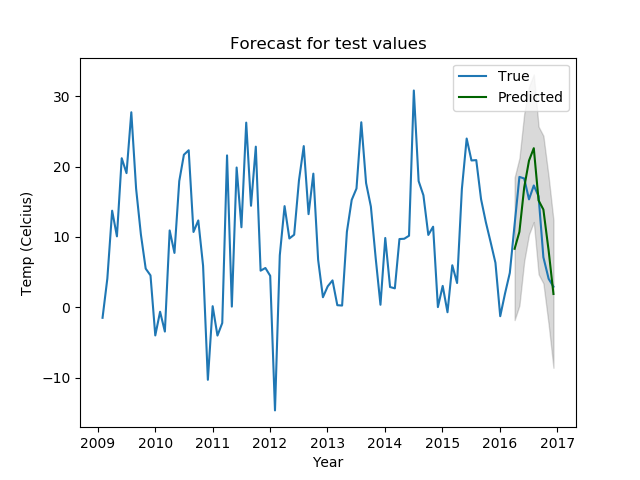
These plots are not bad; the predicted values all fall in the confidence range and the seasonal patterns are captured well, too.
That being said, we have lost all granularity in the data while trying to make the algorithm work for us with limited compute. We need other methods.
You can learn more about Autoregressive models in this article.
Smoothing Methods
Exponential smoothing methods are often used in time series forecasting. They utilize the exponential window function to smooth a time series. There are multiple variations of smoothing methods, too.
The simplest form of exponential smoothing can be thought of this way:
$$ s_{0} = x_{0} \\ s_{t} = \alpha x_{t} + (1 - \alpha) s_{t - 1} = s_{t - 1} + \alpha (x_{t} - s_{t - 1}) $$
Where $x$ represents the original values, $s$ represents the predicted values, and $\alpha$ is the smoothing factor, where:
$$ 0 \leq \alpha \leq 1 $$
Which means that the smoothed statistic $s_{t}$ is the weighted average of the current real value and the smoothed value of the previous time step, with the previous time step value added as a constant.
For a greater smoothing of the curve, the value of the smoothing factor (somewhat counterintuitively) needs to be lower. Having $\alpha = 1$ is equivalent to the original time series. The smoothing factor can be found by using the mthod of least squares, where you minimize the following.
$$ (s_{t} - x_{t + 1})^2 $$
The smoothing method is called exponential smoothing because when you recursively apply the formula:
$$ s_{t} = \alpha x_{t} + (1 - \alpha) s_{t - 1} $$
You get:
$$ s_{t} = \alpha \sum_{i = 0}^{t} (1 - \alpha)^i x_{t - i} $$
Which is a geometric progression, i.e. a discrete version of an exponential function.
We will implement three variants of exponential smoothing: Simple Exponential Smoothing, Holt's Linear Smoothing, and Holt's Exponential Smoothing. We will try to find out how changing the hyperparamters of the different smoothing algorithms changes our forecasting output, and see which one works best for us.
from statsmodels.tsa.holtwinters import SimpleExpSmoothing, Holt
from statsmodels.tsa.holtwinters import ExponentialSmoothing
from sklearn.metrics import mean_squared_error
def exponential_smoothing(df, smoothing_level=0.2):
model = SimpleExpSmoothing(np.asarray(df))
model._index = pd.to_datetime(df.index)
fit = model.fit(smoothing_level=smoothing_level)
return fit
def holts_linear_smoothing(df, smoothing_level=0.3, smoothing_slope=0.05):
model = Holt(np.asarray(df))
model._index = pd.to_datetime(df.index)
fit = model.fit(smoothing_level=smoothing_level, smoothing_slope=smoothing_slope)
return fit
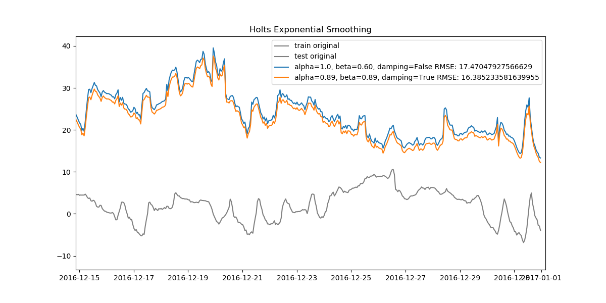
def holts_exponential_smoothing(df, trend=None, damped=False, seasonal=None, seasonal_periods=None):
model = ExponentialSmoothing(np.asarray(df), trend=trend, seasonal=seasonal, damped=damped, seasonal_periods=seasonal_periods)
model._index = pd.to_datetime(df.index)
fit = model.fit()
return fitAll three models have different hyperparameters which we will test out using grid search. We will also return the RMSE values for us to compare and get the best model.
import numpy as np

def smoothing_experiments(train, test, params, method):
    methods = ['simpl_exp', 'holts_lin', 'holts_exp']
    models = {}
    preds = {}
    rmse = {}
    if method == methods[0]:
        for s in params['smoothing_level']:
            models[s] = exponential_smoothing(train, smoothing_level=s)
            preds[s] = models[s].predict(start=1,end=len(test))
            preds[s] -= preds[s][0]
            preds[s] += train.values[-1]
            rmse[s] = np.sqrt(mean_squared_error(test, preds[s]))
    elif method == methods[1]:
        for sl in params['smoothing_level']:
            for ss in params['smoothing_trend']:
                models[(sl,ss)] = holts_linear_smoothing(train, smoothing_level=sl, smoothing_slope=ss)
                preds[(sl,ss)] = models[(sl,ss)].predict(start=1,end=len(test))
                preds[(sl,ss)] -= preds[(sl,ss)][0]
                preds[(sl,ss)] += train.values[-1]
                rmse[(sl,ss)] = np.sqrt(mean_squared_error(test, preds[(sl,ss)]))
    elif method == methods[2]:
        for t in params['trend']:
            for d in params['damped_trend']:
                models[(t,d)] = holts_exponential_smoothing(train, trend=t, damped=d)
                preds[(t,d)] = models[(t,d)].predict(start=1,end=len(test))
                preds[(t,d)] -= preds[(t,d)][0]
                preds[(t,d)] += train.values[-1]
                rmse[(t,d)] = np.sqrt(mean_squared_error(test, preds[(t,d)]))
    fig, ax = plt.subplots(figsize=(12, 6))
    ax.plot(train.index, train.values, color="gray", label='train original')
    ax.plot(test.index, test.values, color="gray", label='test original')
    for p, f, r in zip(list(preds.values()),list(models.values()),list(rmse.values())):
        if method == methods[0]:
            ax.plot(test.index, p, label="alpha="+str(f.params['smoothing_level'])[:3]+" RMSE: "+str(r))
            ax.set_title("Simple Exponential Smoothing")
            ax.legend();
        elif method == methods[1]:
            ax.plot(test.index, p, label="alpha="+str(f.params['smoothing_level'])[:4]+", beta="+str(f.params['smoothing_trend'])[:4]+" RMSE: "+str(r))
            ax.set_title("Holts Linear Smoothing")
            ax.legend();
        elif method == methods[2]:
            ax.plot(test.index, p,
                    label="alpha="+str(f.params['smoothing_level'])[:4]+", beta="+str(f.params['smoothing_trend'])[:4]+ ", damping="+str(True if f.params['damping_trend']>0 else False)+" RMSE: "+str(r),
                    )
            ax.set_title("Holts Exponential Smoothing")
            ax.legend();
    plt.show()
    return models, preds, rmse
Now we run the experiments with different hyperparameters.
# defining the parameters for hyperparameter search
simpl_exp_params = {
    'smoothing_level': [0.2, 0.3, 0.5],
}

holts_lin_params = {
    'smoothing_level': [0.2, 0.3, 0.5],
    'smoothing_trend': [0.05, 0.1, 0.2],
}

holts_exp_params = {
    'trend': ['add'],
    'damped_trend': [False, True],
}

df = pd.read_csv('jena_climate_2009_2016.csv')

series = df['T (degC)'][5::6]
time = pd.to_datetime(df.pop('Date Time'), format='%d.%m.%Y %H:%M:%S')[5::6]
series.index = time

train = series[:-int(len(series)/10)]
test = series[-int(len(series)/10):]


simpl_exp_models, simpl_exp_preds, simpl_exp_rmse = smoothing_experiments(train, test, simpl_exp_params, 'simpl_exp')
holts_lin_models, holts_lin_preds, holts_lin_rmse = smoothing_experiments(train, test, holts_lin_params, 'holts_lin')
holts_exp_models, holts_exp_preds, holts_exp_rmse = smoothing_experiments(train, test, holts_exp_params, 'holts_exp')
Let's look at how our plots turned out.
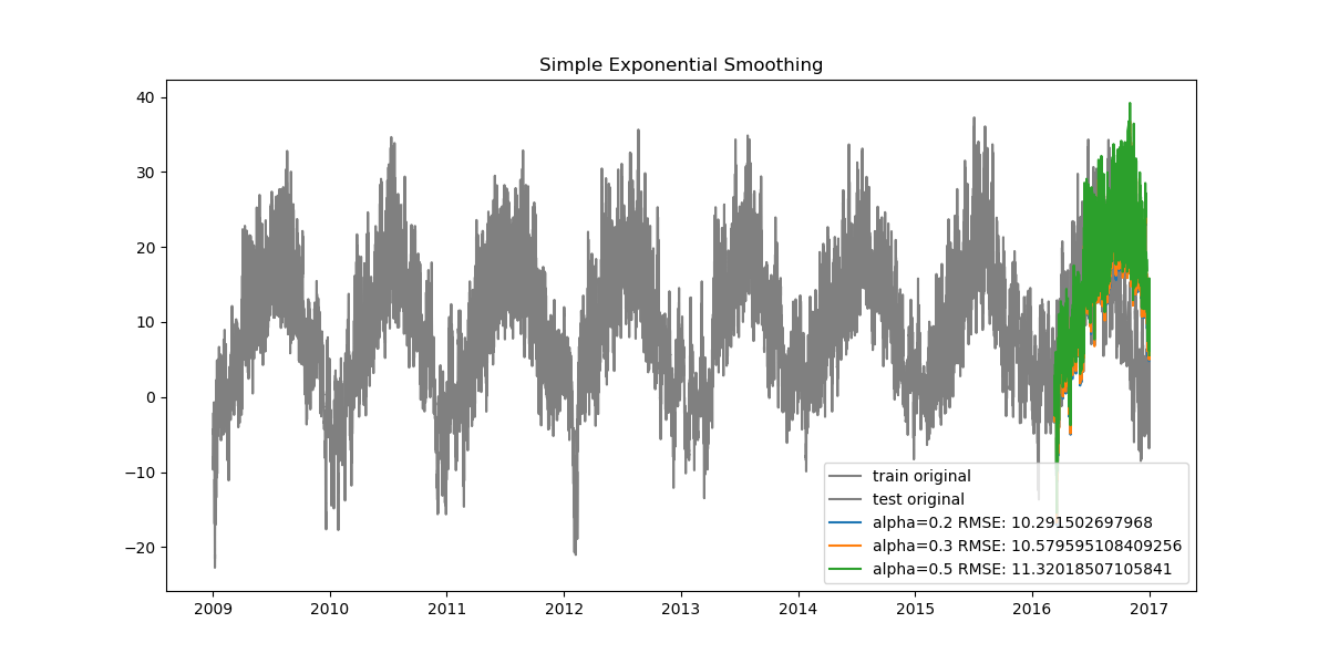
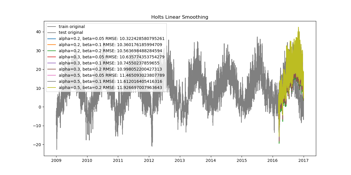
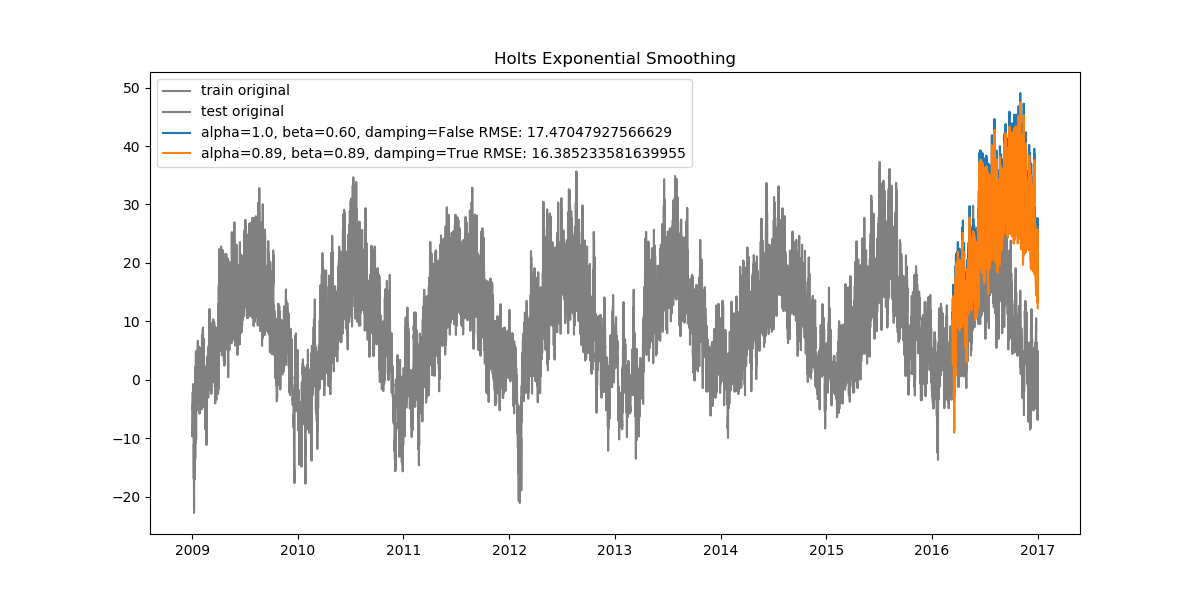
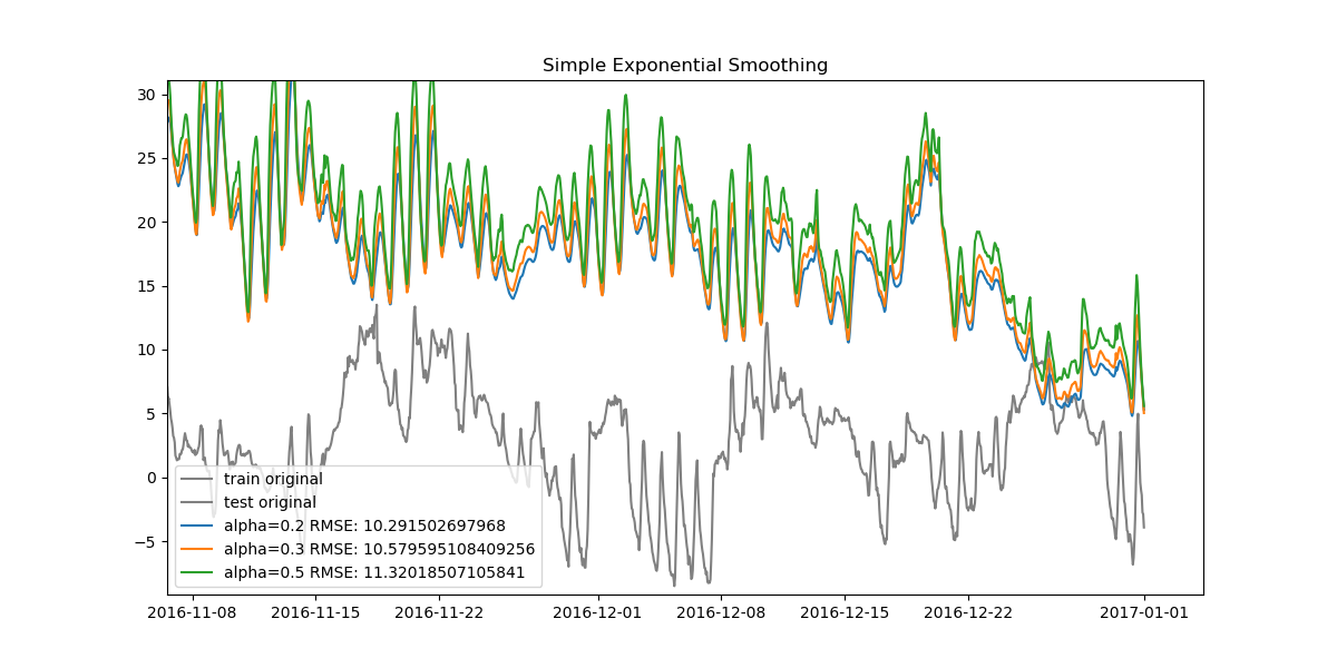
Since our data is very dense, when looked at from start to finish the plots can seem cluttered. Let's also look at how the data looks when zoomed in.
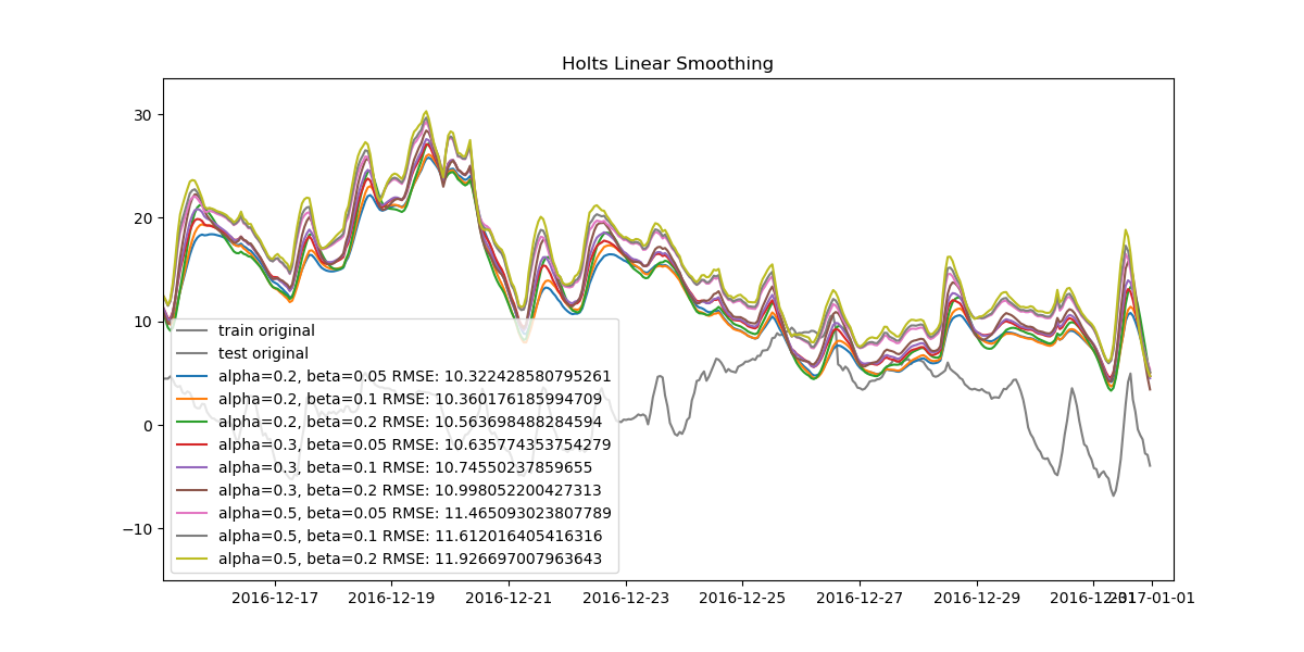
We can find the best model for all three methods and compare them, too.
# find the best model based on the RMSE values
def get_best_model(rmse):
    min_rmse = min(rmse.values())
    best = [key for key in rmse if rmse[key] == min_rmse]
    return best[0]

best1 = get_best_model(simpl_exp_rmse)
best2 = get_best_model(holts_lin_rmse)
best3 = get_best_model(holts_exp_rmse)

# get plots for all the exponential smoothing best models
plt.figure(figsize=(12,6))
plt.plot(train.index, train.values, color='gray')
plt.plot(test.index, test.values, color='gray')
plt.title('Simple and Holt Smoothing Forecast')

preds = simpl_exp_preds[best1]
rmse = np.sqrt(mean_squared_error(test, preds))
plt.plot(test.index[:len(preds)], preds, color='red', label='preds - simple exponential smoothing - RMSE - {}'.format(rmse))
plt.legend()

preds = holts_lin_preds[best2]
rmse = np.sqrt(mean_squared_error(test, preds))
plt.plot(test.index[:len(preds)], preds, color='green', label='preds - holts linear smoothing - RMSE - {}'.format(rmse))
plt.legend()

preds = holts_exp_preds[best3]
rmse = np.sqrt(mean_squared_error(test, preds))
plt.plot(test.index[:len(preds)], preds, color='orange', label='preds - holts exponential smoothing - RMSE - {}'.format(rmse))
plt.legend()

plt.show()
We find the following results.
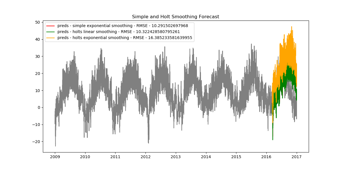
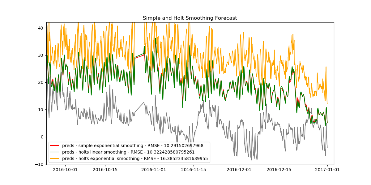
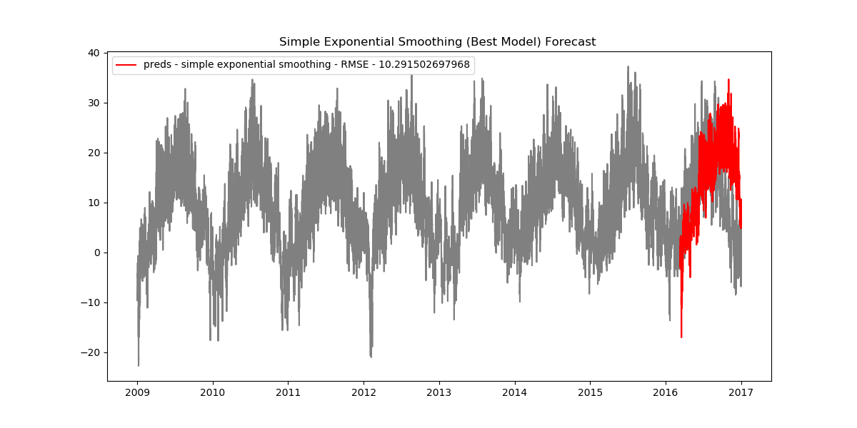
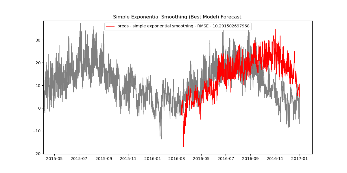
As it turns out, the simple exponential model has the smallest RMSE value, thus making it the best model we have.
plt.figure(figsize=(12,6))
plt.plot(train.index, train.values, color='gray')
plt.plot(test.index, test.values, color='gray')
plt.title('Simple Exponential Smoothing (Best Model) Forecast ')

preds = simpl_exp_preds[best1]
rmse = np.sqrt(mean_squared_error(test, preds))
plt.plot(test.index[:len(preds)], preds, color='red', label='preds - simple exponential smoothing - RMSE - {}'.format(rmse))
plt.legend()
plt.show()
You can find and run the code for this series of articles here.
Conclusion
In this part of the series we looked mainly at autoregressive models, explored moving average terms, lag orders, differencing, accounting for seasonality, and their implementation which includes grid search-based hyperparameter selection. We then moved onto exponential smoothing methods, looking into simple exponential smoothing, Holt's linear and exponential smoothing, grid search-based hyperparameter selection with a discrete user-defined search space, best model selection, and inference.
In the next part, we will look at how to create features, train models, and make predictions for classical machine learning algorithms like linear regression, random forest regression, and also deep learning algorithms like LSTMs.
Hope you enjoyed the read.