
In the first part of this series, Introduction to Time Series Analysis, we covered the different properties of a time series, autocorrelation, partial autocorrelation, stationarity, tests for stationarity, and seasonality.
In the second part we introduced time series forecasting. We looked at how we can make predictive models that can take a time series and predict how the series will move in the future. Specifically, we looked at autoregressive models and exponential smoothing models.
In this final part of the series, we will look at machine learning and deep learning algorithms used for time series forecasting, including linear regression and various types of LSTMs.
You can find the code for this series and run it for free on a Gradient Community Notebook from the ML Showcase.
Bring this project to life
Introduction
We will be using the same data we used in the previous articles for our experiments, namely the weather data from Jena, Germany. You can download it using the following command.
wget https://storage.googleapis.com/tensorflow/tf-keras-datasets/jena_climate_2009_2016.csv.zipOpen the zip file and load the data into a Pandas dataframe.
import pandas as pd

df = pd.read_csv('jena_climate_2009_2016.csv')

time = pd.to_datetime(df.pop('Date Time'), format='%d.%m.%Y %H:%M:%S')
series = df['T (degC)'][5::6]
series.index = time[5::6]
Before we are able to build our models, we will have to do some basic feature engineering. We create a matrix of lagged values out of the time series using a window of a specific length. Say the window length is 4. Then your array will look something like:
$$ \begin{vmatrix} x_{t} & x_{t - 1} & x_{t - 2} & x_{t - 3} \\ x_{t -1} & x_{t - 2} & x_{t - 3} & x_{t - 4} \\ .. & .. & .. & .. \\ .. & .. & .. & .. \\ x_{4} & x_{3} & x_{2} & x_{1} \\ x_{3} & x_{2} & x_{1} & x_{0} \end{vmatrix} $$
In our prediction models, the last column would serve as the labels and the rest of the columns as the predictors.
In our case, it would make sense to chose a window size of one day because of the seasonality in daily data.
import numpy as np

# function for generating the lagged matrix
def split_sequence(sequence, window_size):
    X = []
    y = []
    # for all indexes
    for i in range(len(sequence)):
        end_idx = i + window_size
        # exit condition
        if end_idx > len(sequence) - 1:
            break
        # get X and Y values
        seq_x, seq_y = sequence[i:end_idx], sequence[end_idx]
        X.append(seq_x)
        y.append(seq_y)
    return np.array(X), np.array(y)


train = series[:-int(len(series)/10)]
test = series[-int(len(series)/10):]
X_train, y_train = split_sequence(train, window_size=24)
Modelling Time Series Using Regression
Regression algorithms try to find the line of best fit for a given dataset. The linear regression algorithm tries to minimize the value of the sum of the squares of the differences between the observed value and predicted value. OLS regression has several underlying assumptions called Gauss-Markov assumptions. Gauss-Markov assumptions for cross-sectional data include the following:
- The parameters (the value of the slope of the best fit line in a two-variable regression line, for example) should be linear.
- $X$ and $Y$ should be random variables.
- No perfect collinearity between multiple independent variables.
- The covariance of the residual term and the independent variables should be $0$, or in other words, the residual term is endogenous.
- Homoscedasticity for the residual term, i.e. the variance in the residual term should not change with a change in the independent variable.
- No autocorrelation in the residual terms.
For time series data, we cannot satisfy the assumption that independent variables are all random variables since different columns are coming from the same process. To compensate for that the assumptions on autocorrelation, homoscedasticity and endogeneity are more strict.
Let's see what a simple regression model might get us.
import statsmodels.api as sm

# train Ordinary Least Squares model
X_train = sm.add_constant(X_train)
model = sm.OLS(y_train, X_train)
result = model.fit()

print(result.summary())
The model summary looks like this:
                            OLS Regression Results
==============================================================================
Dep. Variable:                      y   R-squared:                       0.992
Model:                            OLS   Adj. R-squared:                  0.992
Method:                 Least Squares   F-statistic:                 3.376e+05
Date:                Fri, 22 Jan 2021   Prob (F-statistic):               0.00
Time:                        13:53:01   Log-Likelihood:                -70605.
No. Observations:               63058   AIC:                         1.413e+05
Df Residuals:                   63033   BIC:                         1.415e+05
Df Model:                          24
Covariance Type:            nonrobust
==============================================================================
                 coef    std err          t      P>|t|      [0.025      0.975]
------------------------------------------------------------------------------
const          0.0317      0.005      6.986      0.000       0.023       0.041
x1            -0.1288      0.004    -32.606      0.000      -0.137      -0.121
x2             0.0669      0.007     10.283      0.000       0.054       0.080
x3             0.0571      0.007      8.707      0.000       0.044       0.070
x4             0.0381      0.007      5.793      0.000       0.025       0.051
x5             0.0081      0.007      1.239      0.216      -0.005       0.021
x6             0.0125      0.007      1.905      0.057      -0.000       0.025
x7            -0.0164      0.007     -2.489      0.013      -0.029      -0.003
x8             0.0062      0.007      0.939      0.348      -0.007       0.019
x9            -0.0069      0.007     -1.056      0.291      -0.020       0.006
x10            0.0148      0.007      2.256      0.024       0.002       0.028
x11            0.0029      0.007      0.436      0.663      -0.010       0.016
x12            0.0129      0.007      1.969      0.049    5.75e-05       0.026
x13           -0.0018      0.007     -0.272      0.786      -0.015       0.011
x14           -0.0033      0.007     -0.502      0.616      -0.016       0.010
x15           -0.0180      0.007     -2.731      0.006      -0.031      -0.005
x16           -0.0029      0.007     -0.437      0.662      -0.016       0.010
x17            0.0157      0.007      2.382      0.017       0.003       0.029
x18           -0.0016      0.007     -0.239      0.811      -0.014       0.011
x19           -0.0006      0.007     -0.092      0.927      -0.013       0.012
x20           -0.0062      0.007     -0.949      0.343      -0.019       0.007
x21           -0.0471      0.007     -7.163      0.000      -0.060      -0.034
x22           -0.0900      0.007    -13.716      0.000      -0.103      -0.077
x23           -0.2163      0.007    -33.219      0.000      -0.229      -0.204
x24            1.3010      0.004    329.389      0.000       1.293       1.309
==============================================================================
Omnibus:                    11270.669   Durbin-Watson:                   2.033
Prob(Omnibus):                  0.000   Jarque-Bera (JB):           181803.608
Skew:                          -0.388   Prob(JB):                         0.00
Kurtosis:                      11.282   Cond. No.                         197.
==============================================================================
A Durbin-Watson value greater than 2 suggests that our series has no autocorrelation.
Checking for normality can be done with the following tests:
from scipy import stats

# get values of the residuals
residual = result.resid

# run tests and get the p values
print('p value of Jarque-Bera test is: ', stats.jarque_bera(residual)[1])
print('p value of Shapiro-Wilk test is: ', stats.shapiro(residual)[1])
print('p value of Kolmogorov-Smirnov test is: ', stats.kstest(residual, 'norm')[1])
We get the following results:
p value of Jarque-Bera test is:  0.0
p value of Shapiro-Wilk test is:  0.0
p value of Kolmogorov-Smirnov test is:  0.0
Assuming a significance level of 0.05, all three tests suggest that our series is not normally distributed.
For heteroscedasticity, we will use the following tests:
import statsmodels.stats.api as sms

print('p value of Breusch–Pagan test is: ', sms.het_breuschpagan(result.resid, result.model.exog)[1])
print('p value of White test is: ', sms.het_white(result.resid, result.model.exog)[1])
We get the following results:
p value of Breusch–Pagan test is:  2.996182722643564e-246
p value of White test is:  0.0
Assuming a significance level of 0.05, the two tests suggest that our series is heteroscedastic.
Our series is neither homoscedastic nor normally distributed. Lucky for us, unlike OLS, generalized least squares accounts for these residual errors.
import statsmodels.api as sm

# train Ordinary Least Squares model
X_train = sm.add_constant(X_train)
model = sm.GLS(y_train, X_train)
result = model.fit()

print(result.summary())
The results summary looks like this.
                            GLS Regression Results
==============================================================================
Dep. Variable:                      y   R-squared:                       0.992
Model:                            GLS   Adj. R-squared:                  0.992
Method:                 Least Squares   F-statistic:                 3.376e+05
Date:                Fri, 22 Jan 2021   Prob (F-statistic):               0.00
Time:                        13:25:24   Log-Likelihood:                -70605.
No. Observations:               63058   AIC:                         1.413e+05
Df Residuals:                   63033   BIC:                         1.415e+05
Df Model:                          24
Covariance Type:            nonrobust
==============================================================================
                 coef    std err          t      P>|t|      [0.025      0.975]
------------------------------------------------------------------------------
const          0.0317      0.005      6.986      0.000       0.023       0.041
x1            -0.1288      0.004    -32.606      0.000      -0.137      -0.121
x2             0.0669      0.007     10.283      0.000       0.054       0.080
x3             0.0571      0.007      8.707      0.000       0.044       0.070
x4             0.0381      0.007      5.793      0.000       0.025       0.051
x5             0.0081      0.007      1.239      0.216      -0.005       0.021
x6             0.0125      0.007      1.905      0.057      -0.000       0.025
x7            -0.0164      0.007     -2.489      0.013      -0.029      -0.003
x8             0.0062      0.007      0.939      0.348      -0.007       0.019
x9            -0.0069      0.007     -1.056      0.291      -0.020       0.006
x10            0.0148      0.007      2.256      0.024       0.002       0.028
x11            0.0029      0.007      0.436      0.663      -0.010       0.016
x12            0.0129      0.007      1.969      0.049    5.75e-05       0.026
x13           -0.0018      0.007     -0.272      0.786      -0.015       0.011
x14           -0.0033      0.007     -0.502      0.616      -0.016       0.010
x15           -0.0180      0.007     -2.731      0.006      -0.031      -0.005
x16           -0.0029      0.007     -0.437      0.662      -0.016       0.010
x17            0.0157      0.007      2.382      0.017       0.003       0.029
x18           -0.0016      0.007     -0.239      0.811      -0.014       0.011
x19           -0.0006      0.007     -0.092      0.927      -0.013       0.012
x20           -0.0062      0.007     -0.949      0.343      -0.019       0.007
x21           -0.0471      0.007     -7.163      0.000      -0.060      -0.034
x22           -0.0900      0.007    -13.716      0.000      -0.103      -0.077
x23           -0.2163      0.007    -33.219      0.000      -0.229      -0.204
x24            1.3010      0.004    329.389      0.000       1.293       1.309
==============================================================================
Omnibus:                    11270.669   Durbin-Watson:                   2.033
Prob(Omnibus):                  0.000   Jarque-Bera (JB):           181803.608
Skew:                          -0.388   Prob(JB):                         0.00
Kurtosis:                      11.282   Cond. No.                         197.
==============================================================================
We can get our predictions as follows:
X_test = sm.add_constant(X_test)

y_train_preds = result.predict(X_train)
y_test_preds = result.predict(X_test)

from matplotlib import pyplot as plt

# indexes start from 24 due to the window size we chose
plt.plot(pd.Series(y_train, index=train[24:].index), label='train values')
plt.plot(pd.Series(y_test, index=test[24:].index), label='test values')
plt.plot(pd.Series(y_train_preds, index=train[24:].index), label='train predictions')
plt.plot(pd.Series(y_test_preds, index=test[24:].index), label='test predictions')
plt.xlabel('Date time')
plt.ylabel('Temp (Celcius)')
plt.title('Forecasts')
plt.legend()
plt.show()
Our predictions look like this:
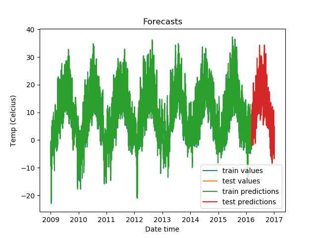
Zoomed in, the predictions on the test set look like this.
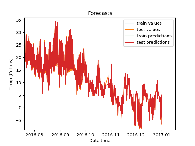
The predictions look highly accurate!
Now we will look at some other approaches for time series and see if they perform as well as regression does.
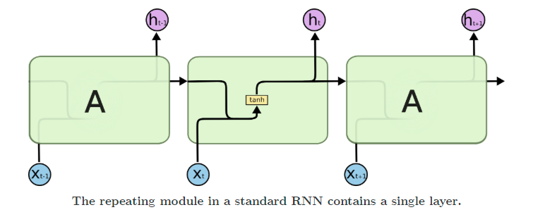
Modelling Time Series With Recurrent Networks
RNNs, or recurrent neural networks, have a hidden layer that acts as a memory function that takes into account the previous timesteps while calculating what the next value in the sequence (the present timestep) should be.
Recurrent networks suffer from issues like vanishing and exploding gradients. To solve for these, LSTMs came into being. They add multiple gates, like input and forget gates, to avoid the problem of exploding or vanishing gradients.
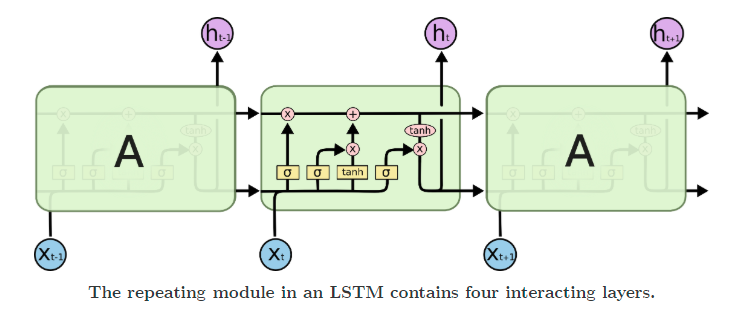
Other ways of dealing with the problem include gradient clipping and identity initialization.
We will look at different LSTM-based architectures for time series predictions. We will use PyTorch for our implementation.
We will test Vanilla LSTMs, Stacked LSTMs, Bidirectional LSTMs, and LSTMs followed by a fully-connected layer.
Before we do that, let's prepare our tensor datasets and dataloaders.
First we load the data.
df = pd.read_csv('jena_climate_2009_2016.csv')

time_vals = pd.to_datetime(df.pop('Date Time'), format='%d.%m.%Y %H:%M:%S')
series = df['T (degC)'][5::6]
series.index = time_vals[5::6]
Then we create our test and train splits.
# train test split
train = series[:-int(len(series)/10)]
train_idx = train.index
test = series[-int(len(series)/10):]
test_idx = test.index
We use the StandardScaler from scikit-learn to scale our data.
from sklearn.preprocessing import StandardScaler

scaler = StandardScaler()
train = pd.Series(scaler.fit_transform(train.values.reshape(-1, 1))[:, 0], index=train_idx)
test = pd.Series(scaler.transform(test.values.reshape(-1, 1))[:, 0], index=test_idx)
And we use the lag matrix generation function we defined earlier to create our test and train datasets.
window_size = 24

X_train, y_train = split_sequence(train, window_size=window_size)
X_test, y_test = split_sequence(test, window_size=window_size)
Then we convert all of this data into tensors, and subsequently a Torch TensorDataset and DataLoaders.
import torch
from torch.utils.data import TensorDataset, DataLoader


# convert train and test data to tensors
X_train = torch.tensor(X_train, dtype=torch.float)
y_train = torch.tensor(y_train, dtype=torch.float)
X_test = torch.tensor(X_test, dtype=torch.float)
y_test = torch.tensor(y_test, dtype=torch.float)

# use torch tensor datasets
train_data = TensorDataset(X_train, y_train)
test_data = TensorDataset(X_test, y_test)

# get data loaders
batch_size = 32
train_dataloader = DataLoader(train_data, shuffle=True, batch_size=batch_size)
test_dataloader = DataLoader(test_data, shuffle=False, batch_size=batch_size)
Let's define the module that we will use to define our neural network architecture. We will make provisions for:
- Vanilla LSTM
- Stacked LSTM
- Bidirectional LSTM
- One fully-connected layer after the LSTM
from torch import nn


class DenseLSTM(nn.Module):
    def __init__(self, input_dim, hidden_dim, lstm_layers=1, bidirectional=False, dense=False):
        super(DenseLSTM, self).__init__()
        self.input_dim = input_dim
        self.hidden_dim = hidden_dim
        self.layers = lstm_layers
        self.bidirectional = bidirectional
        self.dense = dense
        # define the LSTM layer
        self.lstm = nn.LSTM(input_size=self.input_dim,
                            hidden_size=self.hidden_dim,
                            num_layers=self.layers,
                            bidirectional=self.bidirectional)
        self.act1 = nn.ReLU()
        # change linear layer inputs depending on if lstm is bidrectional
        if not bidirectional:
            self.linear = nn.Linear(self.hidden_dim, self.hidden_dim)
        else:
            self.linear = nn.Linear(self.hidden_dim * 2, self.hidden_dim)
        self.act2 = nn.ReLU()
        # change linear layer inputs depending on if lstm is bidrectional and extra dense layer isn't added
        if bidirectional and not dense:
            self.final = nn.Linear(self.hidden_dim * 2, 1)
        else:
            self.final = nn.Linear(self.hidden_dim, 1)


    def forward(self, inputs, labels=None):
        out = inputs.unsqueeze(1)
        out, h = self.lstm(out)
        out = self.act1(out)
        if self.dense:
            out = self.linear(out)
            out = self.act2(out)
        out = self.final(out)
        return out
Now for the training function.
import time

def fit(model, optimizer, criterion):
    print("{:<8} {:<25} {:<25} {:<25}".format('Epoch',
                                          'Train Loss',
                                          'Test Loss',
                                          'Time (seconds)'))
    for epoch in range(epochs):
        model.train()
        start = time.time()
        epoch_loss = []
        # for batch in train data
        for step, batch in enumerate(train_dataloader):
            # make gradient zero to avoid accumulation
            model.zero_grad()
            batch = tuple(t.to(device) for t in batch)
            inputs, labels = batch
            # get predictions
            out = model(inputs)
            out.to(device)
            # get loss
            loss = criterion(out, labels)
            epoch_loss.append(loss.float().detach().cpu().numpy().mean())
            # backpropagate
            loss.backward()
            optimizer.step()
        test_epoch_loss = []
        end = time.time()
        model.eval()
        # for batch in validation data
        for step, batch in enumerate(test_dataloader):
            batch = tuple(t.to(device) for t in batch)
            inputs, labels = batch
            # get predictions
            out = model(inputs)
            # get loss
            loss = criterion(out, labels)
            test_epoch_loss.append(loss.float().detach().cpu().numpy().mean())
        print("{:<8} {:<25} {:<25} {:<25}".format(epoch+1,
                                                  np.mean(epoch_loss),
                                                  np.mean(test_epoch_loss),
                                                  end-start))
Now we can begin the training. We define the hidden layer sizes, epochs, loss function, and which optimizer we will use. Then we train the model and plot the predictions.
device = torch.device(type='cuda')
hidden_dim = 32
epochs = 5
# vanilla LSTM
model = DenseLSTM(window_size, hidden_dim, lstm_layers=1, bidirectional=False, dense=False)
model.to(device)
# define optimizer and loss function
optimizer = torch.optim.Adam(model.parameters())
criterion = nn.MSELoss()
# initate training
fit(model, optimizer, criterion)
# get predictions on validation set
model.eval()
preds = []
for step, batch in enumerate(test_dataloader):
batch = tuple(t.to(device) for t in batch)
inputs, labels = batch
out = model(inputs)
preds.append(out)
preds = [x.float().detach().cpu().numpy() for x in preds]
preds = np.array([y for x in preds for y in x])
# plot data and predictions and applying inverse scaling on the data
plt.plot(pd.Series(scaler.inverse_transform(y_train.float().detach().cpu().numpy().reshape(-1, 1))[:, 0], index=train[window_size:].index), label='train values')
plt.plot(pd.Series(scaler.inverse_transform(y_test.float().detach().cpu().numpy().reshape(-1, 1))[:, 0], index=test[:-window_size].index), label='test values')
plt.plot(pd.Series(scaler.inverse_transform(preds.reshape(-1, 1))[:, 0], index=test[:-window_size].index), label='test predictions')
plt.xlabel('Date time')
plt.ylabel('Temp (Celcius)')
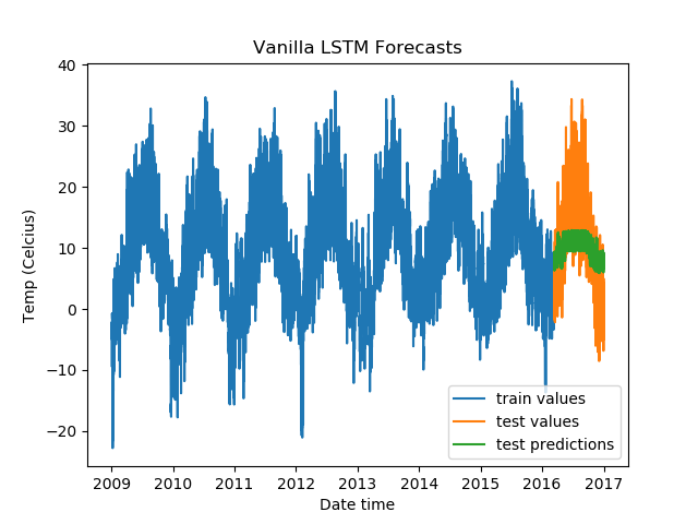
plt.title('Vanilla LSTM Forecasts')
plt.legend()
plt.show()
We get the following results.
Epoch    Train Loss                Test Loss                 Time (seconds)
1        0.9967056512832642        0.7274604439735413        4.000955820083618
2        0.990510106086731         0.566585123538971         4.1188554763793945
3        0.9876610636711121        0.653666079044342         4.1249611377716064
4        0.9871518015861511        0.6488878726959229        4.147826910018921
5        0.9848467707633972        0.5858491659164429        4.120056867599487
To test out other LSTM architectures, you need to change just one line (besides the title of the plots). Test it out on a Gradient Community Notebook with a free GPU. But do make sure to reuse the entire snippet, because you would want to create a new optimizer and loss function instance every time you train a new model, too.
For Stacked LSTMs:
model = DenseLSTM(window_size, hidden_dim, lstm_layers=2, bidirectional=False, dense=False)
The results:
Epoch    Train Loss                Test Loss                 Time (seconds)
1        0.9966062903404236        0.7322613000869751        5.929869890213013
2        0.9892004728317261        0.6665323376655579        5.805717945098877
3        0.9877941608428955        0.650715172290802         5.973452806472778
4        0.9876391291618347        0.6218239665031433        6.097705602645874
5 0.9873654842376709 0.6142457127571106 6.03947639465332 
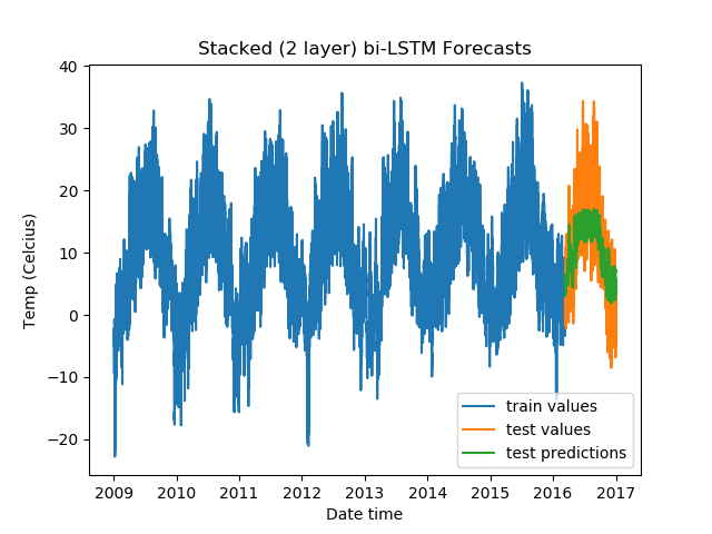
For Stacked Bidirectional LSTMs:
model = DenseLSTM(window_size, hidden_dim, lstm_layers=2, bidirectional=True, dense=False)
The results:
Epoch    Train Loss                Test Loss                 Time (seconds)
1        0.9923199415206909        0.5472036004066467        9.600639343261719
2        0.9756425023078918        0.37495505809783936       9.447819471359253
3        0.9717859625816345        0.3349926471710205        9.493505001068115
4        0.9706487655639648        0.3027298152446747        9.554434776306152
5        0.9707987308502197        0.3214375674724579        9.352233409881592
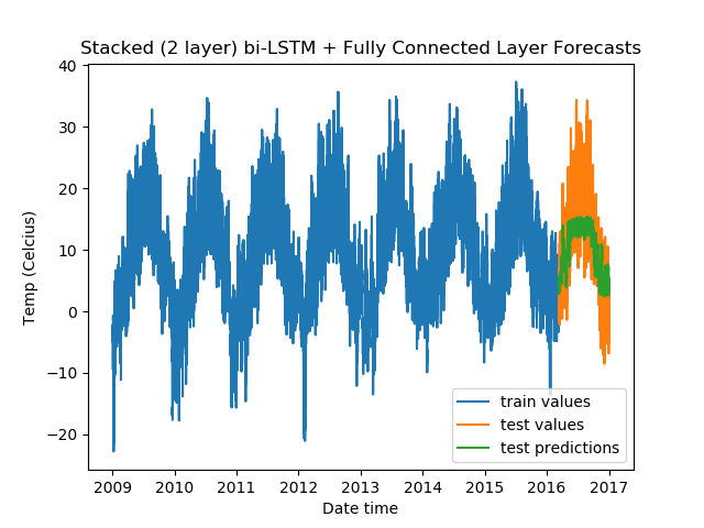
For Stacked Bidirectional LSTMs with a fully-connected layer:
model = DenseLSTM(window_size, hidden_dim, lstm_layers=2, bidirectional=True, dense=True)
And, the results:
Epoch    Train Loss                Test Loss                 Time (seconds)
1        0.9940553903579712        0.5763574838638306        10.142680883407593
2        0.9798027276992798        0.44453883171081543       10.641068458557129
3        0.9713742733001709        0.39177998900413513       10.410093069076538
4        0.9679638147354126        0.35211560130119324       10.61124324798584
5        0.9688050746917725        0.3617672920227051        10.218038082122803
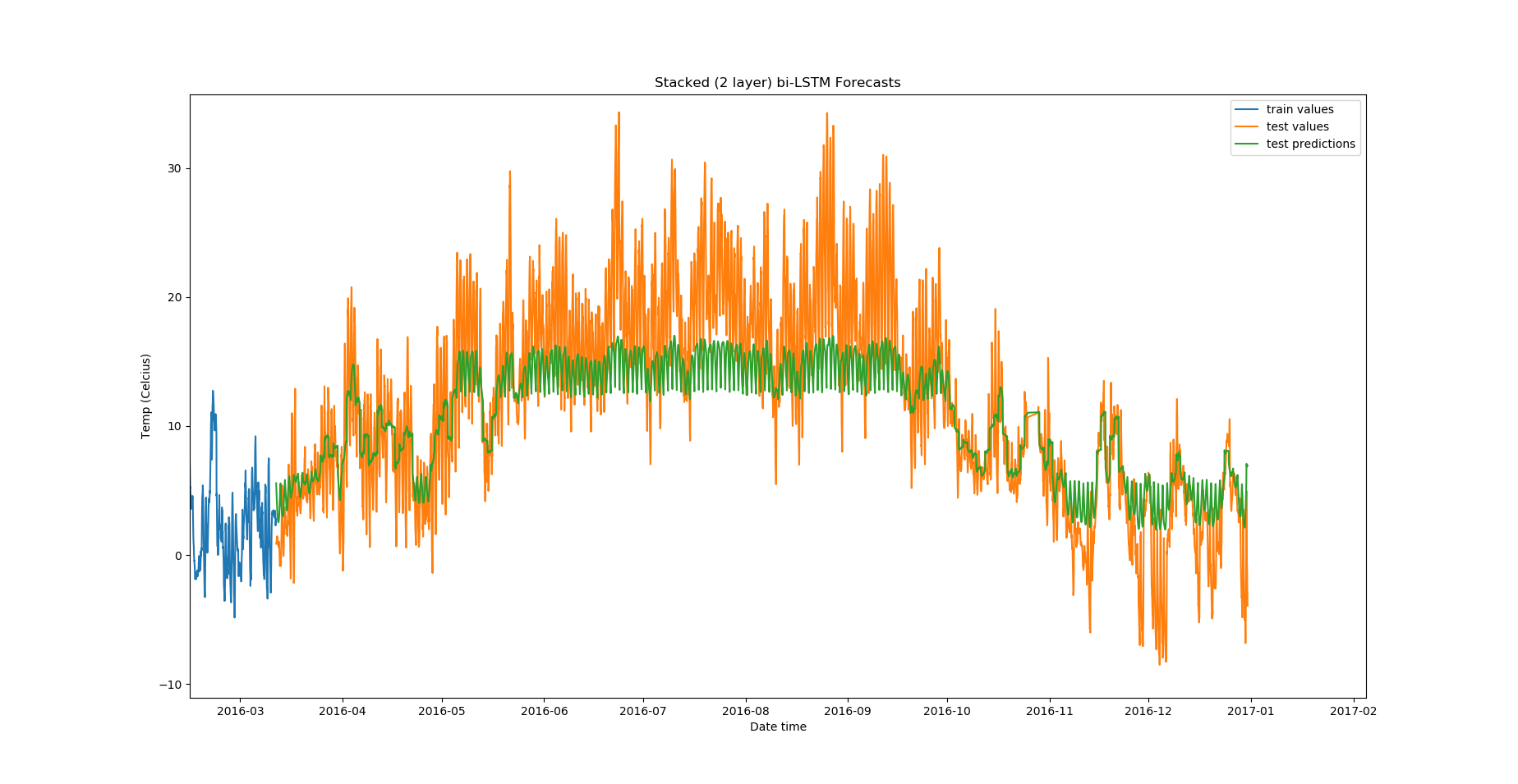
From the validation losses, we find that the third model we tried (2-layer stacked bidirectional LSTM) has the lowest loss, and hence proves to be the best among the models we tested.
Zoomed in, the predictions look like this:
There are a lot of other experiments that you can do in addition to these:
- Train for a greater number of epochs.
- Test out different optimizers.
- Change hyperparameters of our LSTM architectures.
- Add more dense layers.
- Add a 1-D convolutional layer before the LSTM.
- Use batch normalization between layers.
- Test out loss functions other than MSE and MAE.
After these experiments, we still find that our regression model performed a lot better than any of the other methods we tried.
Conclusion
This concludes the final part of our series on time series analysis and forecasting. First we looked at analysis: stationarity tests, making a time series stationary, autocorrelation and partial autocorrelation, frequency analysis, etc. In Part 2 we looked into forecasting methods like AR, MA, ARIMA, SARIMA, and smoothing methods like simple smoothing and Holt's exponential smoothing. In this article we covered forecasting methods that use regression and recurrent networks, like LSTMs.
Over the course of the series, we found that for the data we used, the regression model performed best.
I hope you enjoyed the articles!