
Generative type networks are taking over the world of Artificial Intelligence (AI) at an enormous pace. They are able to create new entities which are almost indistinguishable from the human eye and classify them as real or fake. In previous articles, we have covered one class of these generative type networks in Generative Adversarial Networks (GANs). We have also worked on numerous different types of GAN architectures for creating a multitude of different types of tasks such as deep convolutions GANs (DCGANs), super-resolution images, face generations, and so much more. If you are interested in these projects, I would recommend checking them out on the GANs section of the Paperspace blogs. However, in this article, our primary focus is on the other type of generative type networks in "Autoencoders."
Autoencoders are a blossoming prospect in the field of deep learning similar to its counterpart, GANs. They are useful in a wide array of applications that we will explore further in this article. We will start with some basic introductory material on the field of autoencoders, then proceed to break down some of the essential intricacies related to this topic. Once we have a decent understanding of the relevant concepts, we will construct a few variations of autoencoders to analyze and experiment with their performances accordingly. Finally, we will explore a few of the more critical use-cases where you should consider using these networks for future applications. The code below can be implemented on the Gradient Platform on Paperspace, and it is highly recommended to follow along. Check out the table of contents for a detailed guide on the tasks to follow along with the article.
Bring this project to life
Introduction to Autoencoders:
Autoencoders are a branch of generative neural networks that were primarily designed to encode the input into a compressed and meaningful representation, and then decode it back such that the reconstructed output is as similar as possible to the original input. They make use of learning the efficient coding of unlabeled data to perform the required actions. Apart from the reconstruction of the original image, there are numerous types of autoencoders that perform a variety of tasks. One of the primary types of autoencoders are regularized autoencoders, which aim to prevent the learning of identity functions and encourage the learning of richer representations by improving their ability to capture essential information.
We also have Concrete Autoencoders that are primarily designed for discrete feature selection. They ensure that the latent space only contains the number of features that are specified by the user. Finally, we have one of the more popular variants of autoencoders in variational autoencoders. They find their utility in generative tasks, similar to GANs. They attempt to perform data generation through a probabilistic distribution. We will learn more about variational autoencoders in a separate article, as they are a large enough concept to deserve an article of their own. In this blog, our primary discussion will be on understanding the basic working operation of autoencoders while constructing a couple of deep convolutional autoencoders, and other versions, to analyze their performance on the dimensionality reduction task.
Understanding Autoencoders:
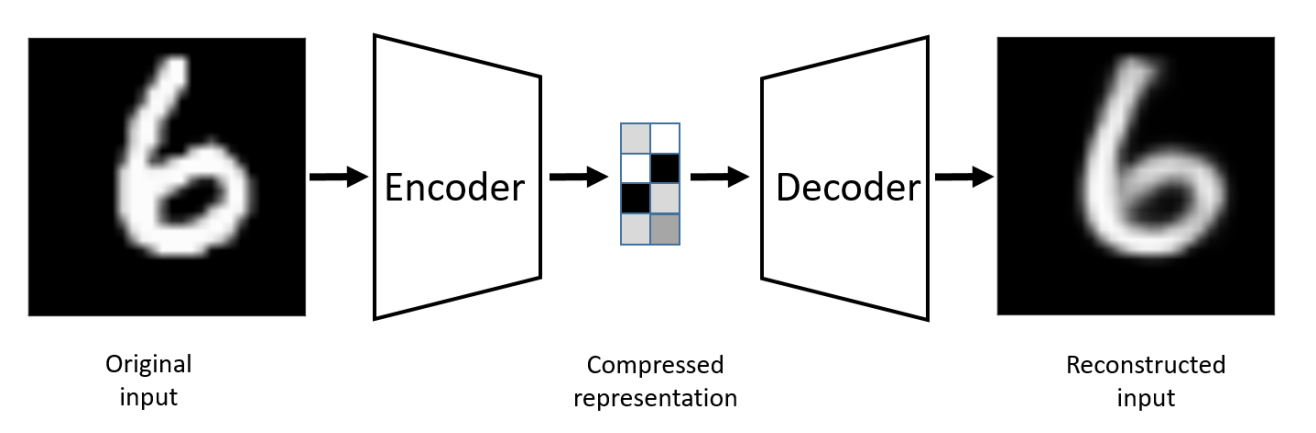
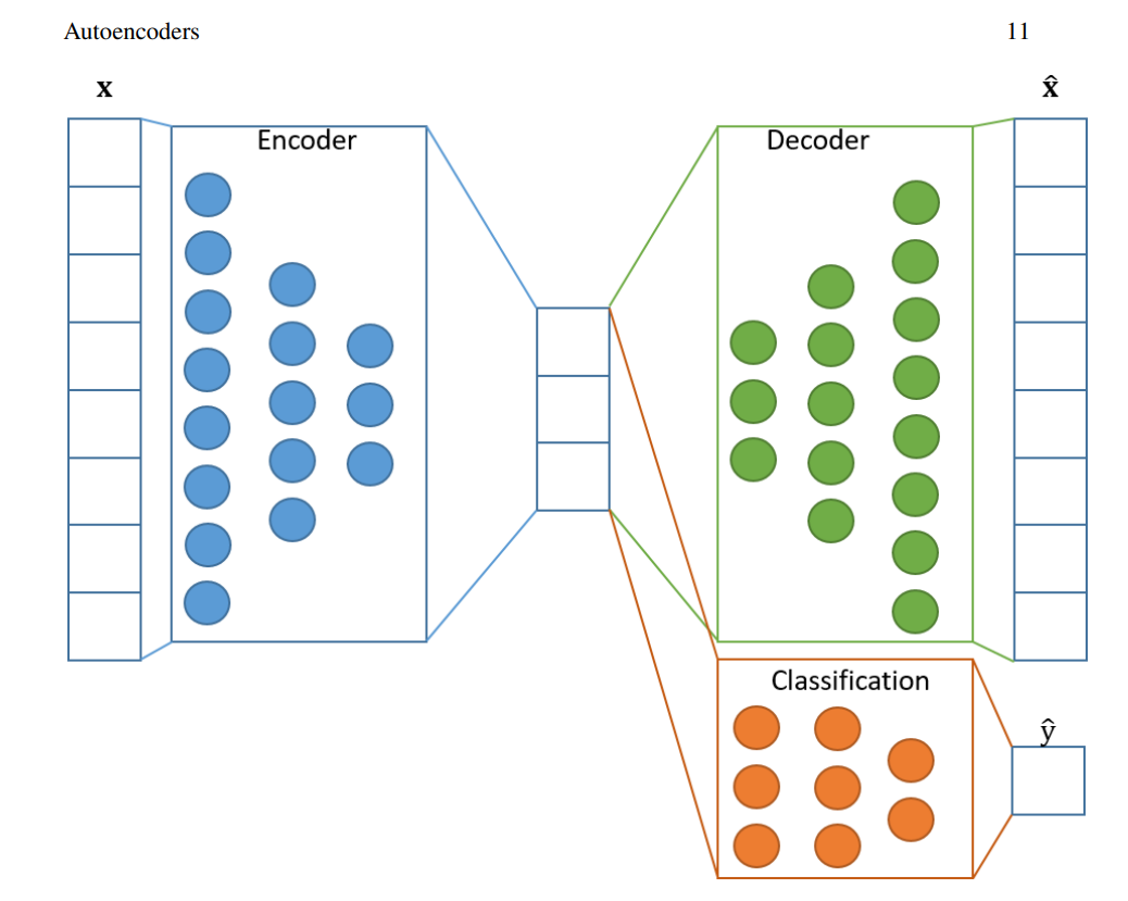
Autoencoders are a unique type of generative network. They consist of an encoder, a latent dimension space, and a decoder. The encoder comprises a neural network architecture that tries to perform the conversion of the higher dimensional data into the lower dimensional vector space. The latent space contains the essential extracted features of the particular image, the data, in a compressed, representative form.
Let us assume that we have a 100 x 100 image that you want to pass through the encoder to reduce the dimensions appropriately. Out of the 10000-pixel dimension space, let us say only about 1000 of these components consist of the data containing the most useful and decisive information, in other words, good quality data. The latent dimensional space of the autoencoder will consist of this lower-dimensional space with the most useful information for reconstruction.
The task of the decoder in the autoencoder is to reconstruct this new data from the existing latent dimension space. Hence, we can see that the regenerated data is an effective reconstruction of the original sample, despite the loss of some information in the process. Unlike generative adversarial networks, which generate completely new data samples, autoencoders primarily do not perform the same function. Therefore, most beginners might be under a common misconception about autoencoders as they wonder about their true purpose; especially when we are just reconstructing the original sample at the price of some small information loss.
In most cases, we are primarily concerned with leveraging the encoder and latent dimensional space for a variety of applications. These are notably denoising of an image, anomaly detection, and other similar tasks. The decoder is usually a pathway for us to visualize the quality of the reconstructed outputs. The autoencoders can be considered a "smarter" version of dimensionality reduction techniques, such as principal component analysis (PCA). We will further break down the significance of these autoencoders in the applications section of the article. For now, let's focus on the practical implementation of these autoencoders with some codes and deep learning.
Deep Convolutional Autoencoders (Approach-1):
There are several methods of constructing the architecture of the autoencoders. In the first two approaches, we will look at a couple of deep convolutional methods that we can implement to solve projects. I will be working with both the Fashion data and MNIST data available in TensorFlow and Keras. These will be our main deep learning frameworks for the construction of these projects. We have covered both these libraries in immense detail in our previous articles. If you aren't familiar with these, I would recommend checking them out from the following link for TensorFlow and the following link for Keras. Let us now begin the construction of the autoencoder models.
Importing the essential libraries:
The first step is to import all the essential libraries that are required to construct the autoencoder model for the particular project. Here, I am importing both the datasets for Fashion MNIST and MNIST dataset. The viewers can feel free to explore their required options. Other necessary imports are the deep learning frameworks provided by Keras and TensorFlow, matplotlib for visualizing the images in both the inputs and returned outputs, and Numpy to help set up our datasets. We will also import some of the required layers for constructing a fully convolutional deep learning network. We will use the Functional API model approach for this task to allow more control over the model structure of the autoencoders. Readers following along can choose either Sequential or model-subclassing (custom method) for approaching the problem as well. Below is the code snippet containing all the desired library imports.
import tensorflow as tf
from tensorflow import keras
import matplotlib.pyplot as plt
import numpy as np
from tensorflow.keras.datasets import fashion_mnist
from tensorflow.keras.datasets import mnist
from tensorflow.keras.layers import Conv2D, MaxPooling2D, UpSampling2D, Input, ZeroPadding2D
from tensorflow.keras.layers import BatchNormalization, LeakyReLU, Activation, Cropping2D, Dense
from tensorflow.keras.models import Model
Preparing The Data:
In the next section of the article, we will prepare our data for this project. Note that the preparation step will vary accordingly for the type of project that you are working on. If you are utilizing a custom dataset, you might require more pre-processing before you pass the images or data through the encoder section of the autoencoder. For our current dataset, it is relatively easy to load the data and segregate them with their respective training and testing entities accordingly. The shape of both the datasets used for this project is 28 x 28, which add up to a total of 784-Dimensional features when flattened as they are grayscale images with a channel of 1. When working with RGB images with 3 channels, like with RGB color images, some variations might occur and must be computed as per the requirement. We will also visualize our data to see the type of images we will be working with for this project.
We can see that the images are not of the highest quality, but they will definitely suffice for an introductory project to autoencoders. We will also normalize the data for both the training and testing data as it would be easier to handle values when they are in the range of 0 to 1 rather than a range of 0 to 255. This practice is quite common when handling such types of data. The code snippet for the normalization is as shown below, and once completed, we can proceed to construct the deep convolutional autoencoder.
# Normalizing the data
x_train = x_train.astype('float32') / 255.0
x_test = x_test.astype('float32') / 255.0
Constructing The Deep Convolutional Autoencoder:
As discussed in the previous section, we know that the autoencoder is comprised mainly of three primary entities, namely the encoder, the latent dimensional, and the decoder. We will now construct the encoder and the decoder neural networks using a deep convolutional approach. This part and the next section will revolve around a couple of methods through which you can construct the encoder and decoder networks to suit your problem and obtain the best results accordingly. Let us get started with the structure of the encoder.
Encoder:
Our architectural build utilizes the functional API structure of TensorFlow, which enables us to quickly adapt to some changes and gives us more control over the particulars of construction. The sequential or model-subclassing methods can also be used to interpret the following code. The first layer in our encoder architecture will consist of the input layer, which will take the shape of the image, in our case a 28 x 28 grayscale pixelated image for both the Fashion and MNIST data. Note that this shape is required for the deep convolutional network. If you plan to use a hidden (or dense) layer type structure for your project, then it is best to flatten the image or convert it into 784-dimension data for further processing.
In the first approach, I have utilized a zero-padding layer to convert the image from the 28 x 28 shape to the 32 x 32 shape. This conversion allows us to get an image that is now a power of 2, and will help us to add more max pooling and convolutional layers. With this change, we can now add four convolutional layers along with the max-pooling layer for each of these convolutions because it will take longer to reach an odd number. We don't want to stride an odd number due to the calculation difficulties. Hence, the encoder neural network architecture makes use of four convolutional layers with the same type of padding and the ReLU activation function. Each of these convolutional layers is followed by a max-pooling layer with a stride of (2, 2) to downsize the image. The encoder architecture code block is as shown in the below snippet.
# Creating the input layer with the full shape of the image
input_layer = Input(shape=(28, 28, 1))

# Note: If utilizing a deep neural network without convolution, ensure that the dimensions are multiplied and converted
#accordingly before passing through further layers of the encoder architecture.

zero_pad = ZeroPadding2D((2, 2))(input_layer)

# First layer
conv1 = Conv2D(16, (3, 3), activation='relu', padding='same')(zero_pad)
pool1 = MaxPooling2D((2, 2), padding='same')(conv1)

# Second layer
conv2 = Conv2D(16, (3, 3), activation='relu', padding='same')(pool1)
pool2 = MaxPooling2D((2, 2), padding='same')(conv2)

# Third layer
conv3 = Conv2D(8, (3, 3), activation='relu', padding='same')(pool2)
pool3 = MaxPooling2D((2, 2), padding='same')(conv3)

# Final layer
conv4 = Conv2D(8, (3, 3), activation='relu', padding='same')(pool3)

# Encoder architecture
encoder = MaxPooling2D((2, 2), padding='same')(conv4)
Decoder:
In the decoder architecture, we will successfully reconstruct our data and finish the entire autoencoder structure. For this reconstruction, the model will require four layers that will upsample our data as soon as it is passed through the next set of deep convolutional layers. We can also make use of convolutional layers with the ReLU activation function and similar padding for the reconstruction procedure. We will then upsample the convolutional layers to double the size and reach the 32 x 32 desired image size after four sets of building blocks. Finally, we will return the original value of the image from 32 x 32 into 28 x 28 by using the Cropping 2D functionality that is available in TensorFlow. Check the code snippet below for the entire decoder layout.
# First reconstructing decoder layer
conv_1 = Conv2D(8, (3, 3), activation='relu', padding='same')(encoder)
upsample1 = UpSampling2D((2, 2))(conv_1)

# Second reconstructing decoder layer
conv_2 = Conv2D(8, (3, 3), activation='relu', padding='same')(upsample1)
upsample2 = UpSampling2D((2, 2))(conv_2)

# Third decoder layer
conv_3 = Conv2D(16, (3, 3), activation='relu', padding='same')(upsample2)
upsample3 = UpSampling2D((2, 2))(conv_3)

# First reconstructing decoder layer
conv_4 = Conv2D(1, (3, 3), activation='relu', padding='same')(upsample3)
upsample4 = UpSampling2D((2, 2))(conv_4)

# Decoder architecture
decoder = Cropping2D((2, 2))(upsample4)
Compilation and Training:
Our next step is to compile the entire architecture of the encoder. We will create the functional API model with the input layer of the encoder followed by the output layer of the decoder. Once the autoencoder is completed, we will compile the model using the Adam optimizer and mean squared error loss.
We can also view the summary of the model to understand the entire structure of the autoencoder. Below is the code snippet for performing the following actions and the summary.
# Creating and compiling the model

autoencoder = Model(input_layer, decoder)
autoencoder.compile(optimizer='adam', loss='mse')
autoencoder.summary()
Model: "model_1"
Layer (type) Output Shape Param #
input_4 (InputLayer) [(None, 28, 28, 1)] 0
zero_padding2d_2 (ZeroPaddin (None, 32, 32, 1) 0
conv2d_16 (Conv2D) (None, 32, 32, 16) 160
max_pooling2d_10 (MaxPooling (None, 16, 16, 16) 0
conv2d_17 (Conv2D) (None, 16, 16, 16) 2320
max_pooling2d_11 (MaxPooling (None, 8, 8, 16) 0
conv2d_18 (Conv2D) (None, 8, 8, 8) 1160
max_pooling2d_12 (MaxPooling (None, 4, 4, 8) 0
conv2d_19 (Conv2D) (None, 4, 4, 8) 584
max_pooling2d_13 (MaxPooling (None, 2, 2, 8) 0
conv2d_20 (Conv2D) (None, 2, 2, 8) 584
up_sampling2d_6 (UpSampling2 (None, 4, 4, 8) 0
conv2d_21 (Conv2D) (None, 4, 4, 8) 584
up_sampling2d_7 (UpSampling2 (None, 8, 8, 8) 0
conv2d_22 (Conv2D) (None, 8, 8, 16) 1168
up_sampling2d_8 (UpSampling2 (None, 16, 16, 16) 0
conv2d_23 (Conv2D) (None, 16, 16, 1) 145
up_sampling2d_9 (UpSampling2 (None, 32, 32, 1) 0
cropping2d_1 (Cropping2D) (None, 28, 28, 1) 0
Total params: 6,705 | Trainable params: 6,705 | Non-trainable params: 0
Since we will run the autoencoder model for this particular task for about 100 epochs, it is best to utilize some appropriate callbacks. We will use model checkpoint for saving the best weights of the model during training, early stopping with a patience of eight to stop the training after eight continuous epochs of no improvement, the reduced learning rate callback to decrease the learning rate after four epochs of no improvement, and finally, TensorBoard to visualize our progress accordingly. Below is the code snippet for the various callbacks that we will use for the autoencoder project.
# Creating Callbacks

from tensorflow.keras.callbacks import ModelCheckpoint
from tensorflow.keras.callbacks import EarlyStopping
from tensorflow.keras.callbacks import TensorBoard
from tensorflow.keras.callbacks import ReduceLROnPlateau

tensorboad_results = TensorBoard(log_dir='autoencoder_logs_fashion/')

checkpoint = ModelCheckpoint("best_model_fashion.h5", monitor="val_loss", save_best_only=True)

early_stop = EarlyStopping(monitor="val_loss", patience=8, restore_best_weights=False)

reduce_lr = ReduceLROnPlateau(monitor="val_loss", factor=0.2, patience=4, min_lr=0.000001)
In the final step, we will fit the autoencoder model and train it for about 100 epochs to achieve the best possible results. Note that the labels, i.e., the training and test (y-train and y-test) label values, are not required and are disregarded for this task. We will use the training and validation samples with a batch size of 128 to train the model. We will also make use of the pre-defined callbacks and let the model run for 100 epochs. The Gradient platform on Paperspace is a great place to run the following project.
# Training our autoencoder model

autoencoder.fit(x_train, x_train,
                epochs=100,
                batch_size=128,
                shuffle=True,
                validation_data=(x_test, x_test),
                callbacks=[checkpoint, early_stop, tensorboad_results, reduce_lr])
Visualization of Results:
After successfully compiling and training the autoencoder model, the final step is to visualize and analyze the results obtained. Use the predict function of the model to return the predicted values for the test data. Store the predictions in a variable, and use the matplotlib library for visualizing the obtained results. The code snippet for constructing this action is as shown below. I have computed two separate autoencoder models for both the Fashion and MNIST data. The results for both these datasets are represented below.
decoded_imgs = autoencoder.predict(x_test)

n = 10
plt.figure(figsize=(20, 4))
for i in range(1, n + 1):
    # Display original
    ax = plt.subplot(2, n, i)
    plt.imshow(x_test[i].reshape(28, 28))
    plt.gray()
    ax.get_xaxis().set_visible(False)
    ax.get_yaxis().set_visible(False)

    # Display reconstruction
    ax = plt.subplot(2, n, i + n)
    plt.imshow(decoded_imgs[i].reshape(28, 28))
    plt.gray()
    ax.get_xaxis().set_visible(False)
    ax.get_yaxis().set_visible(False)
plt.show()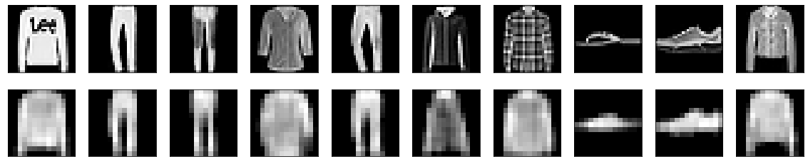
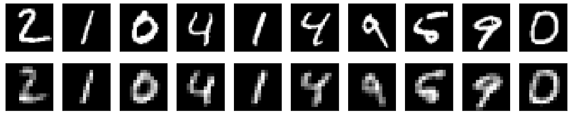
The results obtained after visualizing our predictions were quite decent, especially when compared to other methods such as PCA reconstructions.
While approach-1 gave us a good result, we will try another approach using a similar deep convolutional method to see if it yields a similar, worse, or better result. We will now proceed to the second approach of constructing autoencoders in the next section of the article.
Bring this project to life
Deep Convolutional Autoencoders (Approach-2):
In the second approach for constructing deep convolutional autoencoders, we will use batch normalization layers and Leaky ReLU layers. We will also avoid messing with the original shape of the dataset by avoiding the use of zero padding or cropping 2D layers. Only the encoder and the decoder architecture of the autoencoders are changed in this section. Most of the other parameters and code blocks may remain the same or be modified as per the user's requirement. Let us analyze the encoder architecture to further understand how we will construct this autoencoder.
Encoder:
The encoder architecture contains the input layer, which will take the input of the MNIST images, each of which is a grayscale image with a shape of 28 x 28. The encoder structure will consist of primarily two sets of convolutional networks. Each of these blocks has a convolutional layer with the same padding (and no activation function) followed by a max-pooling layer to perform striding, a Leaky ReLU activation function, and finally, a batch normalization layer to generalize the neural network. After two blocks of these networks, we will pass the information to the decoder to complete the autoencoder architecture.
# Creating the input layer with the full shape of the image
input_layer = Input(shape=(28, 28, 1))

# Note: If utilizing a deep neural network without convolution, ensure that the dimensions are multiplied and converted
# accordingly before passing through further layers of the encoder architecture.

# First layer
conv1 = Conv2D(16, (3, 3), padding='same')(input_layer)
pool1 = MaxPooling2D((2, 2), padding='same')(conv1)
activation1 = LeakyReLU(alpha=0.2)(pool1)
batchnorm1 = BatchNormalization()(activation1)

# Second layer
conv2 = Conv2D(8, (3, 3), padding='same')(batchnorm1)
pool2 = MaxPooling2D((2, 2), padding='same')(conv2)
activation2 = LeakyReLU(alpha=0.2)(pool2)

# Encoder architecture
encoder = BatchNormalization()(activation2)
Decoder:
For the decoder model, we will pass the output from the encoder into a similar reconstruction neural network as used in the encoder model. Instead of utilizing the max-pooling layers for reducing the dimensionality of the data, we will make use of the upsampling layers obtain the original dimensions of the image and reconstruct the data. The code snippet for the decoder architecture is provided below. Once the encoder and decoder blocks are built, the same process as the previous section can be followed to compile, train, and visualize the results.
# First reconstructing decoder layer
conv_1 = Conv2D(8, (3, 3), activation='relu', padding='same')(encoder)
upsample1 = UpSampling2D((2, 2))(conv_1)
activation_1 = LeakyReLU(alpha=0.2)(upsample1)
batchnorm_1 = BatchNormalization()(activation_1)
# Second reconstructing decoder layer
conv_2 = Conv2D(1, (3, 3), activation='relu', padding='same')(batchnorm_1)
upsample2 = UpSampling2D((2, 2))(conv_2)
activation_2 = LeakyReLU(alpha=0.2)(upsample2)
# Encoder architecture
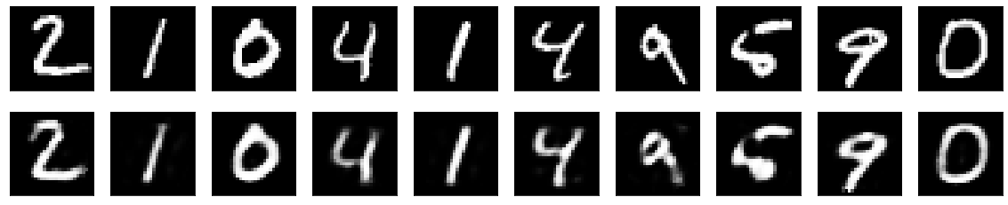
decoder = BatchNormalization()(activation_2)After running the following program for about 100 epochs, I was able to obtain the following results for the MNIST data. Feel free to test the code on other datasets as well and analyze the performance of your neural networks as you desire.
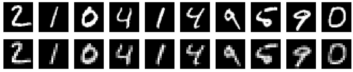
These results seem to look better than the previously generated images. One possible explanation for this is the use of batch normalization layers that help the neural networks to generalize faster and learn better. Also, the final dimensional space reduction, in this case, is much lesser than the first approach. Hence, the recovery stage or the reconstruction seems to look much better because it contains only two real stages of data compression and two stages of data reconstruction. As we compress the data further, there is a higher chance for the information to be lost during the stage of reconstruction. Therefore, each project should be studied and treated according to the desired requirements on a case-by-case basis.
Let us now proceed to discuss some of the other approaches that we can follow for such types of tasks, including other builds of autoencoders.
Discussion on other approaches:
Let's also look at one of the other methods that I utilized for the construction of this project by making use of fully connected layers for both the encoder and the decoder. The first step is to convert the image into a flattened shape of 784 dimensions from the original 28x28 dimensional data and then proceed to train the autoencoder model. Below are the code block and the respective image results obtained for both tasks. You can find similar techniques to see what method suits the particular task best.
x_train = x_train.reshape((len(x_train), np.prod(x_train.shape[1:])))
x_test = x_test.reshape((len(x_test), np.prod(x_test.shape[1:])))

encoding_dim = 32

# Input Sample
input_img = Input(shape=(784,))

# encoder network
encoder = Dense(encoding_dim, activation='relu')(input_img)

# decoder network
decoder = Dense(784, activation='sigmoid')(encoder)

# This model maps an input to its reconstruction
autoencoder = Model(input_img, decoder)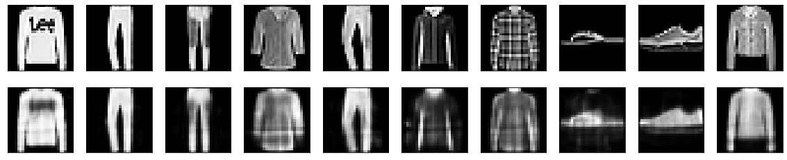
In this article, we have mainly focused on deep convolutional autoencoders. However, there are several different structures that you can implement to construct autoencoders. One such method is to use fully connected dense networks to reproduce and reconstruct the output of the original image. Here is a quick comparison of the difference in reconstruction for an autoencoder to a method like PCA.
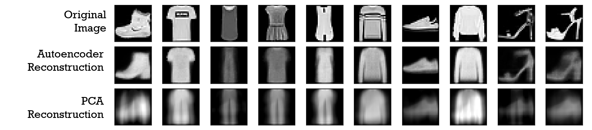
It is noticeable from the above image that autoencoders are one of the most effective methods for the purpose of dimensionality reduction, especially in comparison to some of the other available methods such as PCA, t-Distributed Stochastic Neighbor Embedding (t-SNE), random forests, and other similar techniques. Autoencoders can therefore be considered essential deep learning concept to understand to solve a variety of tasks, especially with regard to computer vision. Let us discuss a few more applications of autoencoders in the next section to understand a deeper understanding of their significance.
Applications of Autoencoders:
Autoencoders are gaining immense popularity due to their wide range of applications in different fields. In this section, we will discuss a few of the awesome capabilities that they possess and the different types of purposes that you can utilize them for in the list below.
- Dimensionality Reduction: One of the primary reasons we use autoencoders is to reduce the dimensionality of the content with minimal information lost, as it is considered to be one of the more superior tools for accomplishing this task with respect to other methods like PCA. This topic is covered in detail in this article.
- Anomaly Detection: Anomaly detection is the process of locating the outliers in the data. Autoencoders tries to minimize the reconstruction error as part of its training, so we can check the magnitude of the reconstruction loss to infer the degree of anomalous data found.
- Image Denoising: Autoencoders do a great job of removing noise from a particular image to represent a more accurate description of the specific data. Old images or blurry images can be denoised with autoencoders to receive a better and realistic representation.
- Feature Extraction: The encoder part of the autoencoders helps to learn the more essential features of the data. Hence, these generative networks hold fantastic utility in extracting the significant information that is critical and required for a particular task.
- Image Generation: Autoencoders can also be used to reconstruct and create modified compressed images. While we have previously discussed that autoencoders are not really utilized for creating a completely new image as they are a reconstruction of the original product, variational autoencoders can be used for the generation of new images. We will discuss more on this topic in future articles.
Conclusion:
Autoencoders have proven to be another revolutionary development in the field of generative type neural networks. They are able to learn most of the essential features of the data provided to them, and reduce the dimensionality while learning most of the critical details of the data provided to them. Most modern autoencoders prioritize the useful properties of the given input, and they have been able to generalize the idea of an encoder and a decoder beyond deterministic functions to stochastic mappings. For further reading, check out the following links - [1] and [2].
In this article, we covered most of the essential aspects required to understand the basic working procedures of autoencoder models. We had a brief introduction to autoencoders and covered a detailed understanding of its generative nature. We also explored a couple of variations of deep convolutional architectures that we can construct to reduce the dimensionality space and reconstruct it accordingly. Apart from our two discussed methods, we had a brief analysis of other methods as well as the performance of other techniques such as PCA. Finally, we looked into a few of the amazing applications of autoencoders and the wide range of capabilities that it possesses.
In future articles, we will focus on some natural language processing (NLP) tasks with Transformers and learn to construct neural networks from scratch without utilizing any deep learning frameworks. We will also further explore Variational Autoencoders in future blogs. Until then, keep exploring!


