Preface
Weights and Biases is a ML Ops platform that has useful features around model tracking, hyperparameter tuning, and artifact saving during model training steps. Integrating with Weights and Biases provides Gradient users access to world-class model experimenting features while taking advantage of Gradient's easy-to-use development platform and access to accelerated hardware.
The goal of this tutorial is to highlight Weights and Biases feature's, and to show how to use them within Gradient to scale up model training. During this tutorial, you will learn to initiate W&B model runs, log metrics, save artifacts, tune hyperparameters, and determine the best performing model. You will then see how to save that model for use with Workflows and Deployments using the Gradient SDK.
The context of this tutorial will be to train and log metrics of ResNet model variations in order to increase accuracy of an image classification model. The dataset that we will be using is a CIFAR-10 dataset, which is a common dataset used to benchmark image classification model performance. The CIFAR-10 dataset will include images belonging to 1 of 10 classes. If you are unfamiliar with ResNet models or the CIFAR-10 dataset, take a look at this walkthrough.
The code used in this tutorial can be found in a GitHub repo here, or follow along the public example in the link below.
Bring this project to life
Basic Commands
Setup
To begin, login or sign up for your Paperspace account here. Once logged in, create a project called Gradient - W&B. In your project, click on the Notebooks tab and then the Create button to pull up the Create a Notebook page shown below.
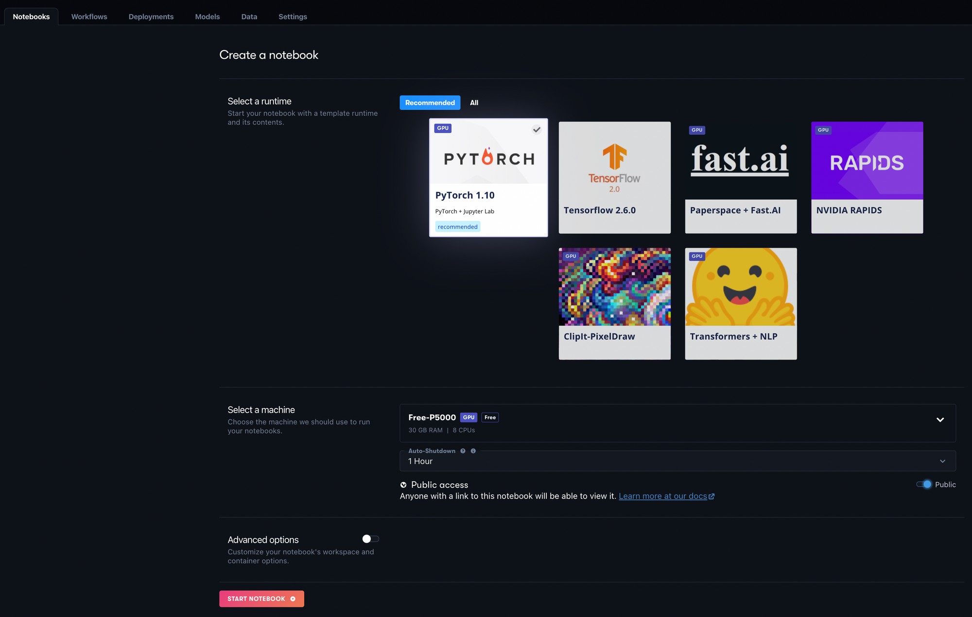
For this project, select the PyTorch 1.10 Runtime and then any GPU instance of your choice under Select a Machine.
Toggle the Advanced options menu and change the Workspace URL to https://github.com/gradient-ai/Gradient-WandB-Tutorial. This is the GitHub repo that will contain the files to run this tutorial. Your Advanced options should look like the image below.
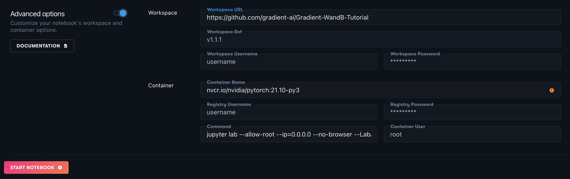
Lastly, click the Start Notebook button and your Notebook will be created. Wait until the Notebook is Running to processed to the following step.
W&B Installation
The code below can be found in the Python Notebook train_model_wandb.ipynb.
The first step in your Notebook will be to install the Weights & Biases Python library into your environment using the command below.
pip install wandb
To import the package you just installed into your Python Notebook, you can use:
import wandb
If you are running wandb through a Python Notebook, you must set the WANDB_NOTEBOOK_NAME environment variable to the relative path of your Notebook. An example of how to do this is below.
import os

os.environ["WANDB_NOTEBOOK_NAME"] = "./train_model_wandb.ipynb"
Login
After installation and setup, you will need to create a Weights & Biases account. You can do that on their site at https://wandb.ai/site.
Once you’ve created a W&B account, you will need to grab your account’s API key in order to integrate your Gradient Notebook with your Weights & Biases account. The API Key can be found in the W&B homepage under Profile → Settings → API Keys. It should be a 40-char string.
Now in your Gradient Notebook, you can login to W&B using the W&B API key found in the above step.
wandb.login(key='your-wandb-api-key')
Initializing a Model Run
After you are logged into your W&B account, you will need to initialize a run before logging any training metrics. To initialize a run, use the following command.
with wandb.init(project="test-project", config=config, name='ResNet18'):
	# Python code below
More details about the wandb.init function can be found here.
The above command will create a project in Weights and Biases called “test-project” (if not already created), and initialize a run that will store the model configuration you passed in with the config object. An example Python config object may look like this:
config={
         "epochs": 10,
         "batch_size": 128,
         "lr": 1e-3,
         }
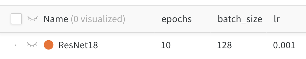
Weights and Biases will track that run and those configurations in the W&B Project Dashboard under the Tables tab. An example of that table is shown below where the model name is used to identify the run and capture the config values.
Log
In the with wand.init() indentation, you will add Python code to log specific model details to W&B during training. Logging data at different steps of the process will create charts that live in your W&B Projects Workspace. Depending on the type of data and frequency that you log during a model run, W&B will create a specific chart type to best visualize that data.
In the script below, the goal is to train a ResNet18 model over 10 epochs, logging the training loss every 50 batches and the validation loss and validation accuracy at the end of each epoch. The script also logs the duration of each epoch and the average epoch run time.
The script is broken up into three steps below. The first step is importing all the necessary libraries and modules. The second step is creating a validate model function that will be used to calculate and log validation metrics. The final step is running the training script that runs through the model training and logging process.
import time
import torch.nn as nn
import torch.optim as optim
import torch

from resnet import resnet18, resnet34
from load_data import load_data
def validate_model(model, valid_dl, loss_func, device):

    # Compute performance of the model on the validation dataset
    model.eval()
    val_loss = 0.
    with torch.inference_mode():
        correct = 0
        for i, (images, labels) in enumerate(valid_dl, 0):
            images, labels = images.to(device), labels.to(device)

            # Forward pass
            outputs = model(images)
            val_loss += loss_func(outputs, labels)*labels.size(0)

            # Compute accuracy and accumulate
            _, predicted = torch.max(outputs.data, 1)
            correct += (predicted == labels).sum().item()

    return val_loss / len(valid_dl.dataset), correct / len(valid_dl.dataset)
model_name = 'ResNet18'

# Initialize W&B run
with wandb.init(project="test-project", config=config, name=model_name):

    # Create Data Loader objects
    trainloader, valloader, testloader = load_data(config)

    # Create ResNet18 Model with 3 channel inputs (colored image) and 10 output classes
    model = resnet18(3, 10)

    # Define loss and optimization functions
    criterion = nn.CrossEntropyLoss()
    optimizer = optim.SGD(model.parameters(), lr=config['lr'], momentum=0.9)

    # Move the model to GPU if accessible
    device = torch.device("cuda:0" if torch.cuda.is_available() else "cpu")
    model.to(device)

    step = 0
    epoch_durations = []
    for epoch in range(config['epochs']):

        epoch_start_time = time.time()
        batch_checkpoint=50
        running_loss = 0.0
        model.train()

        for i, data in enumerate(trainloader, 0):

						# Move the data to GPU if accessible
            inputs, labels = data[0].to(device), data[1].to(device)

            # Zero the parameter gradients
            optimizer.zero_grad()

            # Forward + Backward + Optimize
            outputs = model(inputs)
            loss = criterion(outputs, labels)
            loss.backward()
            optimizer.step()

            running_loss += loss.item()

            # Log every 50 mini-batches
            if i % batch_checkpoint == batch_checkpoint-1:    # log every 50 mini-batches
                step +=1
                print(f'epoch: {epoch + ((i+1)/len(trainloader)):.2f}')
                wandb.log({"train_loss": running_loss/batch_checkpoint, "epoch": epoch + ((i+1)/len(trainloader))}, step=step)

                print('[%d, %5d] loss: %.3f' %
                    (epoch + 1, i + 1, running_loss / batch_checkpoint))

                running_loss = 0.0

        # Log validation metrics
        val_loss, accuracy = validate_model(model, valloader, criterion, device)
        wandb.log({"val_loss": val_loss, "val_accuracy": accuracy}, step=step)
        print(f"Valid Loss: {val_loss:3f}, accuracy: {accuracy:.2f}")

        # Log epoch duration
        epoch_duration = time.time() - epoch_start_time
        wandb.log({"epoch_runtime (seconds)": epoch_duration}, step=step)

        epoch_durations.append(epoch_duration)

    # Log average epoch duration
    avg_epoch_runtime = sum(epoch_durations) / len(epoch_durations)
    wandb.log({"avg epoch runtime (seconds)": avg_epoch_runtime})

print('Training Finished')
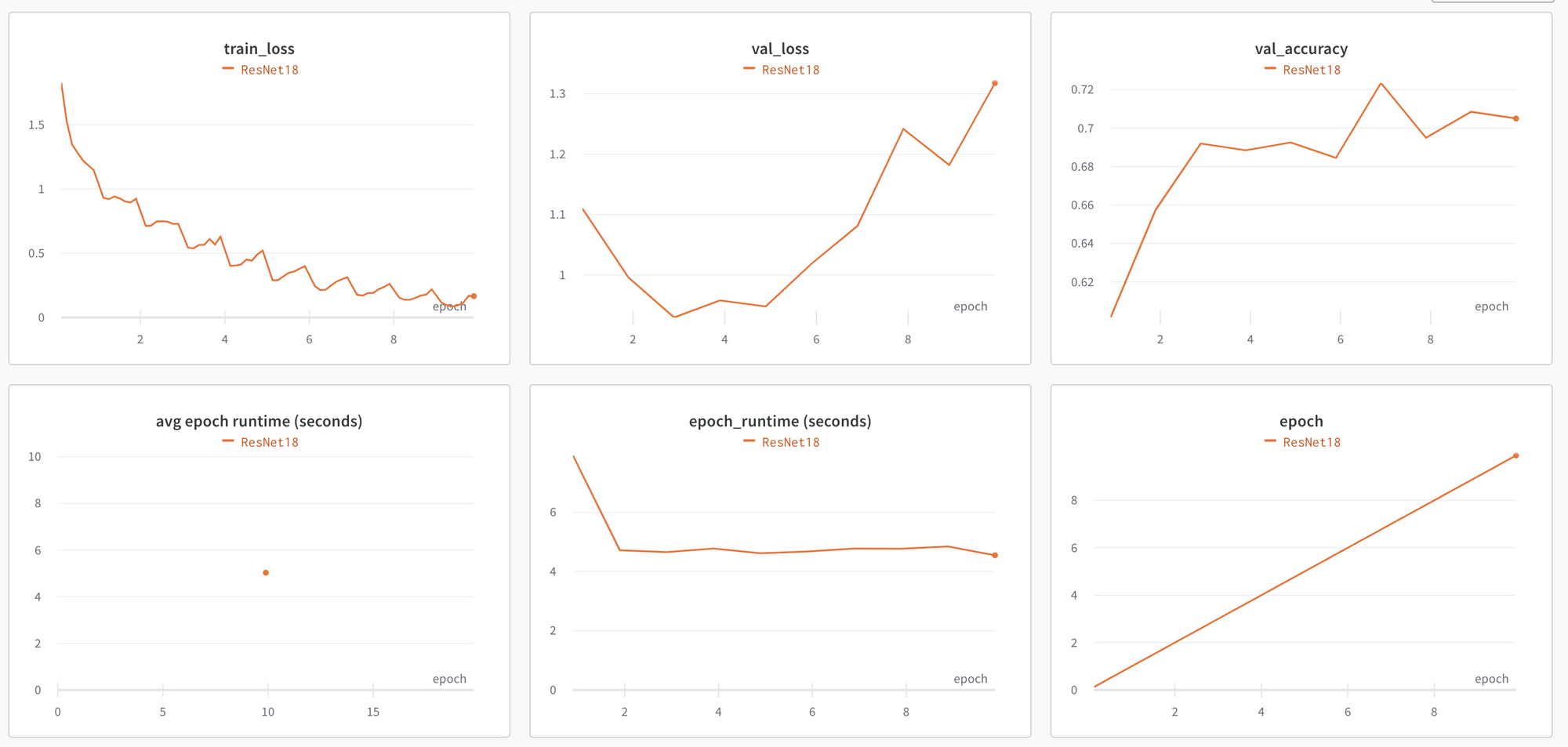
The above script will train the model over 10 epochs (determined from the config), and will log training metrics every 50 batches and at the end of each epoch. At the end of each epoch, the validation loss, validation accuracy, and epoch duration will be logged as well.
All these details will be captured and charted in our Weights & Biases project. You can find this in your Weights & Biases test-project under its Workspace. An example of what this will look like is below.
If you run the same script, but, instead of a ResNet18 model, you use a ResNet34 model, another run will be captured. Both runs can be viewed on the same charts to see how they compare.
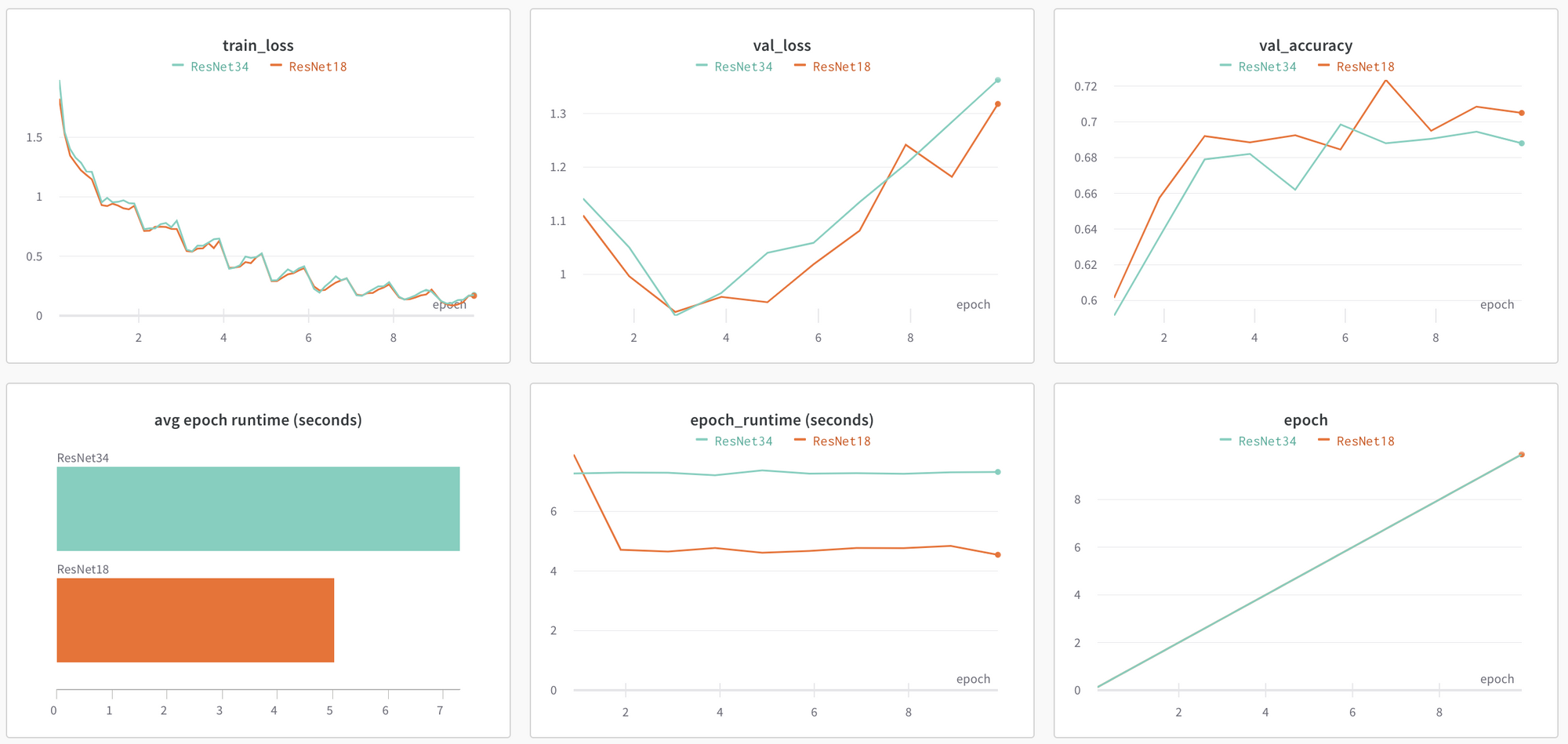
From the charts above, we can tell that the training loss for each of these models are very similar, however the validation accuracy is higher and the Average Epoch Runtime is lower for the ResNet18 model. The epoch runtimes make sense because the ResNet34 model has more layers and therefore has a longer training time. It looks like there may be some overfitting as well as the train loss keeps decreasing but the validation loss starts to climb after the 4th epoch.
Saving Gradient Models
To take full advantage of our models training, we want to be able to do two additional things. First is to save the trained model as a Gradient model artifact. Secondly, we will want to be able to tie a W&B model run to a Gradient model artifact. This is important so that you can take the run results which we’ve seen above and link that to a Gradient model artifact which you can then use in Gradient Workflows and Deployments. For information on Gradient models and how to use them in Workflows and Deployments, please see the Gradient docs.
Below, is a process to save a model as a Gradient artifact, as well as additional code in our training process to log that model name in the Notes of a W&B run.
Before saving a model, you will need to install the Gradient Python SDK. You can do that with the command below.
pip install gradient
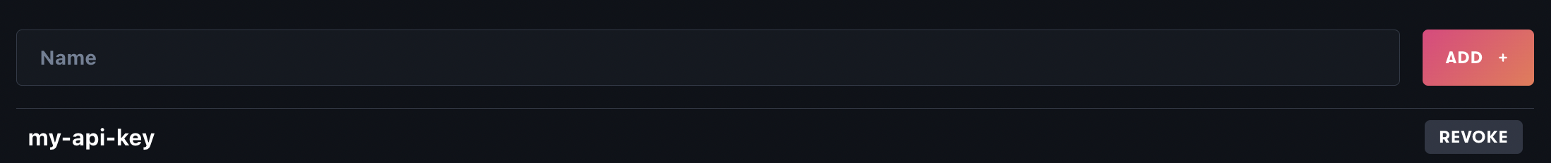
Once the Gradient SDK is installed, you will want to create a Models client to interact with model in your project. To do this you will need to use a Gradient API key. To generate a Gradient API key, on the top right of the Gradient page, select your profile and click Team Settings. Under Team Settings, select the API Keys tab. To generate an API key, enter in an API key name (e.g. my-api-key) and click Add. This will show generate an alpha-numeric string that is your API key. Make sure to save this key somewhere safe as you won’t be able to reference it once you leave the page. Once you have generated and copied your key, you should be able to see it listed like below.
Take the API key from above and use it to create a ModelsClient as seen below.
from gradient import ModelsClient

models_client = ModelsClient(api_key='your-gradient-api-key')
In the upload function, you will need your project ID which is found in the top left corner of your Project Workspace.
Below is the Upload function that takes in a model configuration and model client and saves the model as a Gradient artifact and returns the model name.
def upload_model(config, model_client, model_dir='models'):

    # Create model directory
    if not os.path.exists(model_dir):
        os.makedirs(model_dir)

    # Save model file
    params = [config['model'], 'epchs', str(config['epochs']), 'bs', str(config['batch_size']), 'lr', str(round(config['lr'], 6))]
    full_model_name = '-'.join(params)
    model_path = os.path.join(model_dir, full_model_name + '.pth')
    torch.save(model.state_dict(), model_path)

    # Upload model as a Gradient artifact
    model_client.upload(path=model_path, name=full_model_name, model_type='Custom', project_id='your-project-id')

    return full_model_name
At the end of your training process, you can call that function to save your model and log the model name to your W&B run. Below is an example of what that functionality looks like.
# At the end of your training process

# Upload model artifact to Gradient and log model name to W&B
    full_model_name = upload_model(config, model_client)
    wandb.log({"Notes": full_model_name})

print('Training Finished')
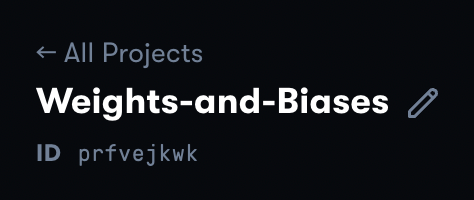
Now we can see the Model saved in your Gradient project under the Models tab.
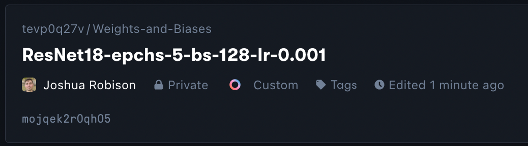
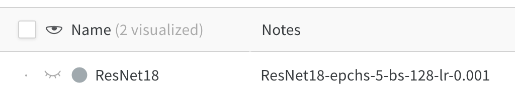
You can also reference the Gradient Model artifact in the Notes section of your W&B run found in the Table tab.
Now you can take your run results, find the best model, find that model in Gradient and use it in your Gradient Workflows and Deployments!
Bring this project to life
Artifacts
Another useful feature of Weights and Biases is the ability to create custom Artifacts that can be saved to your project. As an example, below is a script to create a W&B Table that will be stored as an Artifact in test-project. This table will include pictures of the images from the test dataset, their class label, the model’s predicted class, and the detailed scores of that prediction.
First, you will need to initialize a W&B run and create an artifact. That can be done with the script below.
with wandb.init(project='test-project'):
    artifact = wandb.Artifact('cifar10_image_predictions', type='predictions')
In the with wand.init() indentation, create a table that will store the data described above.
# Classes of images in CIFAR-10 dataset
classes = ('plane', 'car', 'bird', 'cat',
           'deer', 'dog', 'frog', 'horse', 'ship', 'truck')

# Create Data Loader objects
trainloader, valloader, testloader = load_data(config)

# Create columns for W&B table
columns=['image', 'label', 'prediction']
for digit in range(10):
    columns.append("score_" + classes[digit])

# Create W&B table
pred_table = wandb.Table(columns=columns)
Then, run the first test batch through the trained model and capture the prediction, scores, and other data needed.
with torch.no_grad():
    for i, data in enumerate(testloader, 0):

        # Move data to GPU if available
        inputs, labels = data[0].to(device), data[1].to(device)

        # Calculate model outputs and predictions
        outputs = model(in# Create Data Loader objects
        _, predicted = torch.max(outputs.data, 1)

        # Loop through first batch of images and add data to the table
        for j, image in enumerate(inputs, 0):
            pred_table.add_data(wandb.Image(image), classes[labels[j].item()], classes[predicted[j]], *outputs[j])
        break
Lastly, save the table’s data as an Artifact and log it to your W&B project
# Log W&B model artifact
artifact.add(pred_table, "cifar10_predictions")
wandb.log_artifact(artifact)
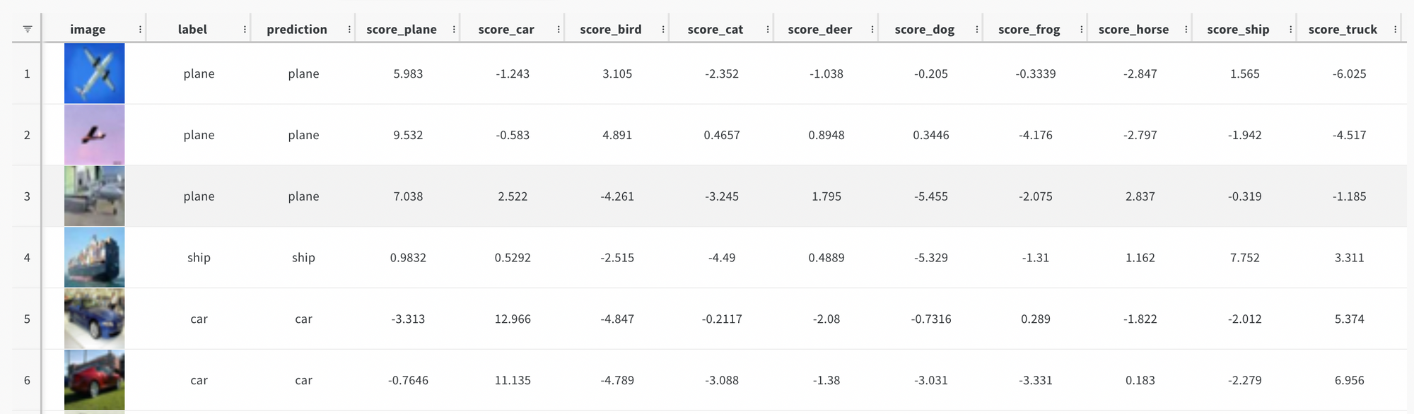
After running the above script, you can navigate to the Artifact by going to the Artifacts section of the W&B Project. Within the Artifact section, click on the Version, the Files tab, and then the JSON file the artifact was saved to. You should then be able to view the table that will look similar to the image below.
Sweeps
Weights & Biases has a hyperparameter tuning feature called Sweeps. Sweeps allow you to specify a model configuration and a training function, and then loops through different combinations of model parameters to identify optimal hyperparameters for your model. We can combine Sweeps with the W&B logging features shown above to log metrics from all these runs to help determine the best performing model.
The first thing you will need to do is create a Sweep config object that will store the hyperparamter options of the model.
sweep_config = {
                'method': 'bayes',
                'metric': {'goal': 'minimize', 'name': 'val_loss'},
                'parameters': {
                    'batch_size': {'values': [32, 128]},
                    'epochs': {'value': 5},
                    'lr': {'distribution': 'uniform',
                                      'max': 1e-2,
                                      'min': 1e-4},
                    'model': {'values': ['ResNet18', 'ResNet34']}
                    }
}
From the above config, you can see 3 high level keys being defined. The first is the method which will define how the Sweep will search for optimal hyperparameters. In the config above, we are using bayesian search.
Next, is the metric key. This will specify what the sweep is trying to optimize. In this case, the goal is to minimize the validation loss.
Lastly, the config has parameters specifications. The parameters included are the hyperparameters for the Sweep to search through. These values can be a single value, a set of values, or a distribution. In this case, all models runs will be trained over 5 epochs, either be one of 2 ResNet models, have a batch size of 32 or 128, and have a learning rate within the specified distribution.
More documentation about Sweep configurations can be found here.
Once the Sweep config is specified, you will need to specify the training function used to train and log the model. The function below should look familiar to the training scripts above however that functionality is moved into a function called train.
def train(config = None):

		# Initialize W&B run
    with wandb.init(project='test-project', config=config):
        config = wandb.config

				# Create Data Loader objects
        trainloader, valloader, testloader = load_data(config)

				# Create a ResNet model depending on the configuration parameters
        if config['model']=='ResNet18':
            model = resnet18(3,10)
        else:
            model = resnet34(3,10)

				# Define loss and optimization functions
        criterion = nn.CrossEntropyLoss()
        optimizer = optim.SGD(model.parameters(), lr=config['lr'], momentum=0.9)

				# Move the model to GPU if accessible
        device = torch.device("cuda:0" if torch.cuda.is_available() else "cpu")
        model.to(device)

        step = 0
        batch_checkpoint=50
        epoch_durations = []
        for epoch in range(config['epochs']):

            epoch_start_time = time.time()
            running_loss = 0.0
            model.train()

            for i, data in enumerate(trainloader, 0):

								# Move the data to GPU if accessible
                inputs, labels = data[0].to(device), data[1].to(device)

                # Zero the parameter gradients
                optimizer.zero_grad()

                # Forward + Backward + Optimize
                outputs = model(inputs)
                loss = criterion(outputs, labels)
                loss.backward()
                optimizer.step()

                running_loss += loss.item()

                # log every 50 mini-batches
                if i % batch_checkpoint == batch_checkpoint-1:    # log every 50 mini-batches
                    step +=1
                    print(f'epoch: {epoch + ((i+1)/len(trainloader)):.2f}')
                    wandb.log({"train_loss": running_loss/batch_checkpoint, "epoch": epoch + ((i+1)/len(trainloader))}, step=step)

                    print('[%d, %5d] loss: %.3f' %
                        (epoch + 1, i + 1, running_loss / batch_checkpoint))

                    running_loss = 0.0

            # Log validation metrics
            val_loss, accuracy = validate_model(model, valloader, criterion, device)
            wandb.log({"val_loss": val_loss, "val_accuracy": accuracy}, step=step)
            print(f"Valid Loss: {val_loss:3f}, accuracy: {accuracy:.2f}")

						# Log epoch duration
            epoch_duration = time.time() - epoch_start_time
            wandb.log({"epoch_runtime (seconds)": epoch_duration}, step=step)

            epoch_durations.append(epoch_duration)

				# Log average epoch duration
        avg_epoch_runtime = sum(epoch_durations) / len(epoch_durations)
        wandb.log({"avg epoch runtime (seconds)": avg_epoch_runtime})

    print('Training Finished')
After the Sweep config and training functionality are define, you can initialize sweep_id and kick off the Sweep by calling wandb.agent().
sweep_id = wandb.sweep(sweep_config, project="test-project")

wandb.agent(sweep_id, function=train, count=10)
This Sweep will kickoff 10 different model runs (set with the count argument) with hyperparemeter values specified in the Sweep config and use Bayesian search to find optimal values for the hyperparameters. These runs will be saved to test-project Dashboard under Sweeps.
Once the Sweep has completed running, you can compare the charts of the runs like below.
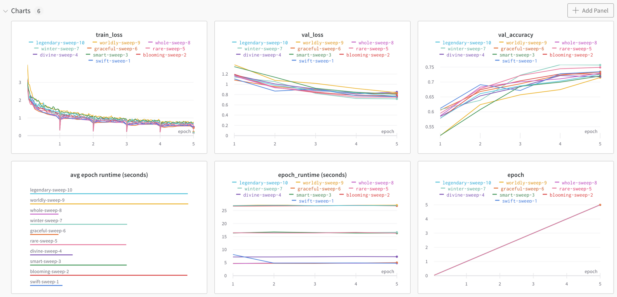
If you zoom into the above chart, you can see the validation accuracy is highest for winter-sweep-7.
Let’s zoom in on the model run details to see what parameters were set for this model run. You can do this by going to the Tables tab.
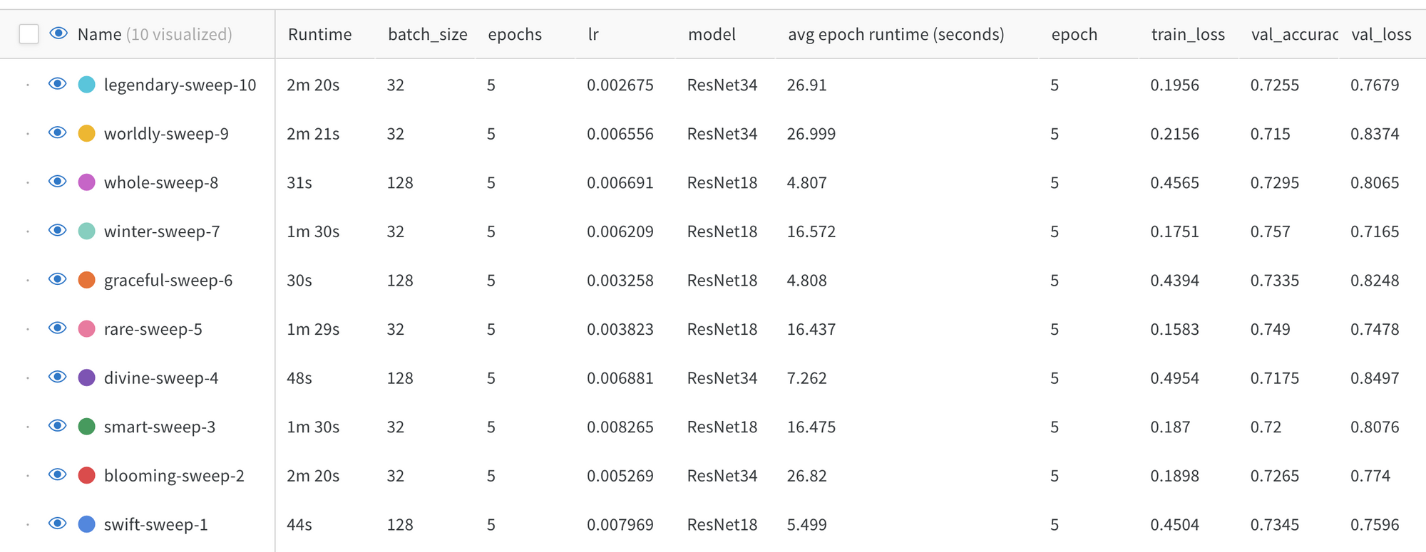
In this example, winter-sweep-7 was run with a ResNet18 model, a batch size of 32 and a learning rate somewhat in the middle of the specified range.
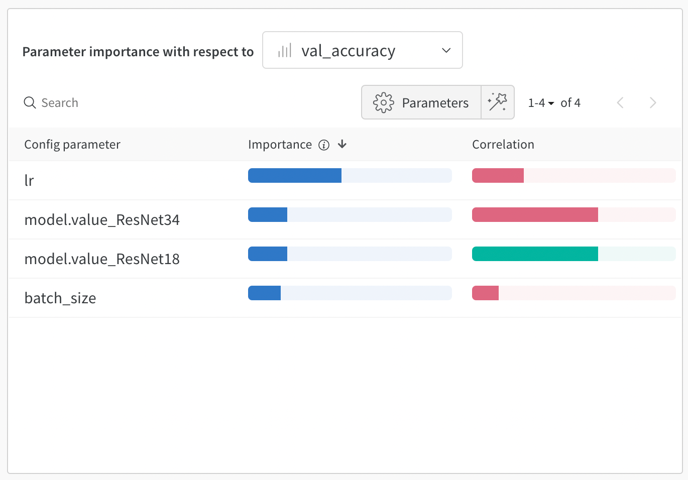
Back in the Sweep Workspace there are a few more helpful charts. The chart below is showing hyperparameter importance with respect to the validation accuracy. Learning rate is the most important hyperparmeter with a negative correlation, meaning the lower the learning rate, the higher the validation accuracy.
The last chart to look at is how the subsequent model runs have improved performance.
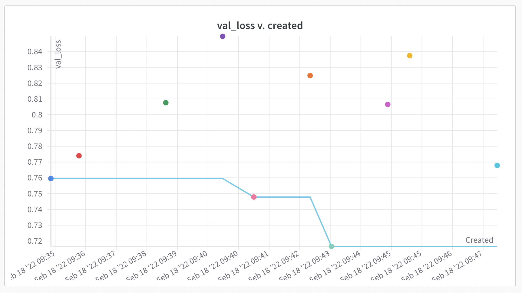
In this example, over the model runs, the Sweep tuned the hyperparameters to improve model performance with respect to validation loss. The 5th and 7th model runs improved the previous model runs’ validation loss with the 7th model run being the best performing of the 10.
Conclusion
Great! Now you should be able to take advantage of some of the features Weights and Biases has to offer for experiment tracking and hyperparameter tuning. You can then store that model artifact in Gradient to be able to reference it inside Gradient Workflows and Deployments. The link to the Gradient documentation including how store model artifacts, using Workflows, and setting up Deployments can be found here.
Again, the needed notebooks and scripts for the above Weights and Biases tutorial to run on Gradient can be found here.