Data Augmentation For Bounding Boxes: Building Input Pipelines for Your Detector

Hello there! This is the fourth and the final part in our series on adapting image augmentation methods for object detection tasks. In the last three posts we have covered a variety of image augmentation techniques such as Flipping, rotation, shearing, scaling and translating. This part is about how to bring it all together and bake it into the input pipeline for your deep network. So, let's get started.

Before you begin, you should be already through the previous articles in the series.

This series has 4 parts.
1. Part 1: Basic Design and Horizontal Flipping
2. Part 2: Scaling and Translation
3. Part 3: Rotation and Shearing
4. Part 4: Baking augmentation into input pipelines

GitHub Repo

Everything from this article and the entire augmentation library can be found in the following Github Repo.

https://github.com/Paperspace/DataAugmentationForObjectDetection

Documentation

The documentation for this project can be found by opening the docs/build/html/index.html in your browser or at this link.

Combing multiple transformations

Now, if you want to apply multiple transformations, you can probably do them by applying them Sequentially, one by one. For example, if I were to apply flipping, followed by scaling and rotating here is how I would accomplish it.  

img, bboxes = RandomHorizontalFlip(1)(img, bboxes)
img, bboxes = RandomScale(0.2, diff = True)(img, bboxes)
img, bboxes = RandomRotate(10)(img, bboxes)

The more the transformations I need to apply, the more longer my code gets.

At this point, We will implement a function that solely combines multiple data augmentations. We will implement it in the same manner as other data augmentations,  only that it takes a list of the class instances of other data augmentations as arguments. Let's write this function.

class Sequence(object):

    """Initialise Sequence object
    
    Apply a Sequence of transformations to the images/boxes.
    
    Parameters
    ----------
    augemnetations : list 
        List containing Transformation Objects in Sequence they are to be 
        applied
    
    probs : int or list 
        If **int**, the probability with which each of the transformation will 
        be applied. If **list**, the length must be equal to *augmentations*. 
        Each element of this list is the probability with which each 
        corresponding transformation is applied
    
    Returns
    -------
    
    Sequence
        Sequence Object 
        
    """
    def __init__(self, augmentations, probs = 1):

        
        self.augmentations = augmentations
        self.probs = probs
        

The self.augmentations attribute stores the list of augmentations we talked about. There is also another attribute, self.probs, which holds the probabilities with which the augmentations of the corresponding instances will be applied.

The __call__ function looks like.

def __call__(self, images, bboxes):
    for i, augmentation in enumerate(self.augmentations):
        if type(self.probs) == list:
            prob = self.probs[i]
        else:
            prob = self.probs
            
        if random.random() < prob:
            images, bboxes = augmentation(images, bboxes)
    return images, bboxes

Now, if we were to apply the same set of transformations as above, we will write.

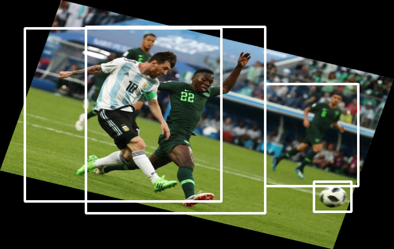
transforms = Sequence([RandomHorizontalFlip(1), RandomScale(0.2, diff = True), RandomRotate(10)])

img, bboxes = transforms(img, bboxes)

Here are the results.

Resizing to an Input Dimension

While a lot of architectures these days are fully convolutional, and hence are size invariant, we often end up choosing a constant input size for sake uniformity and to facilitate putting our images into batches which help in speed gains.

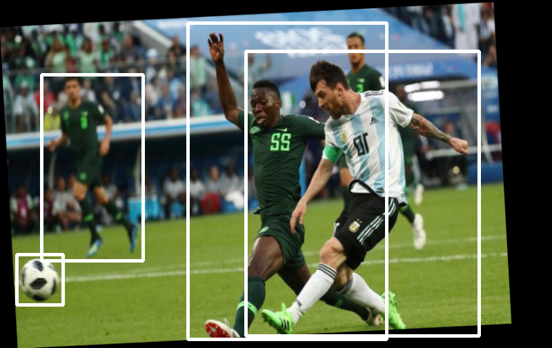
Therefore, we'd like to have a image transform which resizes our images to a constant size as well as our bounding boxes. We also want to maintain our aspect ratio.

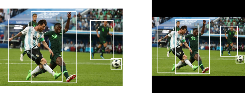
In the example above, the original image is of the size 800 x 505. When we have to resize a rectangular image to a square dimension keeping the aspect ratio constant, we resize the image isotropically (keeping aspect ratio constant) so that longer side is equal to the input dimension.

We implement resizing the same way we resized augmentations.

class Resize(object):
    """Resize the image in accordance to `image_letter_box` function in darknet 
    
    The aspect ratio is maintained. The longer side is resized to the input 
    size of the network, while the remaining space on the shorter side is filled 
    with black color. **This should be the last transform**
    
    
    Parameters
    ----------
    inp_dim : tuple(int)
        tuple containing the size to which the image will be resized.
        
    Returns
    -------
    
    numpy.ndaaray
        Sheared image in the numpy format of shape `HxWxC`
    
    numpy.ndarray
        Resized bounding box co-ordinates of the format `n x 4` where n is 
        number of bounding boxes and 4 represents `x1,y1,x2,y2` of the box
        
    """
    
    def __init__(self, inp_dim):
        self.inp_dim = inp_dim

Before, we build the augmentation logic, we will implement a function called letter_box image, which resizes our image so that the longer side is equal to the input dimension, and the image is centered along the the shorter side.

def letterbox_image(img, inp_dim):
    '''resize image with unchanged aspect ratio using padding'''
    img_w, img_h = img.shape[1], img.shape[0]
    w, h = inp_dim
    new_w = int(img_w * min(w/img_w, h/img_h))
    new_h = int(img_h * min(w/img_w, h/img_h))

    resized_image = cv2.resize(img, (new_w,new_h), interpolation = cv2.INTER_CUBIC)

    #create a black canvas    
    canvas = np.full((inp_dim[1], inp_dim[0], 3), 128)
 
	#paste the image on the canvas
    canvas[(h-new_h)//2:(h-new_h)//2 + new_h,(w-new_w)//2:(w-new_w)//2 + new_w,  :] = resized_image
    
    return canvas

We finally implement the __call__ function.

def __call__(self, img, bboxes):
    w,h = img.shape[1], img.shape[0]
    img = letterbox_image(img, self.inp_dim)


    scale = min(self.inp_dim/h, self.inp_dim/w)
    bboxes[:,:4] *= (scale)

    new_w = scale*w
    new_h = scale*h
    inp_dim = self.inp_dim   

    del_h = (inp_dim - new_h)/2
    del_w = (inp_dim - new_w)/2

    add_matrix = np.array([[del_w, del_h, del_w, del_h]]).astype(int)

    bboxes[:,:4] += add_matrix

    img = img.astype(np.uint8)

    return img, bboxes

Building an Input Pipeline for the COCO Dataset

Now, that we have our augmentations done, and also a way to combine these augmentations, we can actually think about designing an input pipeline that serves us images and annotations from the COCO dataset, with augmentations applied on the fly.

Offline Augmentation vs Online Augmentation

In deep networks, augmentation may be done using two ways. Offline augmentation and online augmentation.

In offline augmentation,  we augment our dataset, create new augmented data and store it on the disk. This can help us multiply our train example by as many times as we want. Since, we have variety of augmentations, applying them stochastically can help us increase our training data many folds before we start to be repetitive.

However, there is one drawback to this method that it isn't as suitable when the size of our data is too big. Consider a training dataset that occupies 50 GB of memory. Augmenting it once alone would make the size go up to 100 GB. This might not be a problem if you have sample disk space, and preferably a SSD or a high-RPM hard disk.

In online augmentations, augmentations are applied just before the images are fed to the neural network. This has a couple of benifits over our previous approach.

1. No space requirements, since the augmentations are done on the fly and we don't need to save augmented training examples.
2. We are getting the noisier versions of the same image every time the image is fed to the neural network. It's well known that minor noise can help neural networks generalise better. Every time a neural network sees the same image, it's a bit different due to the augmentation applied on it. This difference can be thought of as noise, which helps our network generalise better.
3. We get a different augmented dataset each epoch without having to store any extra images.

CPU or GPU?

On a side note, from a computationally point of view, one might wonder whether the CPU or the GPU should be doing the online augmentations during the training loop.

The answer is most likely the CPU. CUDA calls are asynchronous in nature. In simple words, it means that the control of execution returns to the CPU right after the GPU commands (CUDA) are invoked.

Let's break it down how it happens.

1) The CPU keeps reading the code, where it finally reaches a point where it has to invoke the GPU. For example, in PyTorch, the command net = net.cuda() signals to the GPU that variable net needs to be put on the GPU. Any computation made using net now is carried out by the GPU.

2) The CPU makes a CUDA call. This call is asynchronous. This means that the CPU doesn't wait for task specified by the call to be completed by the GPU. The control of execution is immediately returned to CPU and the CPU can start executing the lines of code that follow, while the GPU can do it's thing in the background.

This means that the GPU can carry out the computations in background / parallel now. Modern deep learning libraries make sure that the calls are properly scheduled to ensure our code works properly.  However, this feature is often exploited by deep learning libraries to speed up training. While the GPU is busy executing the forward and the backward passes for the current epoch, the data for the next epoch can be read from the disk and loaded into the RAM in the meantime by the CPU.

So coming back to our question, should the online augmentations be done by the CPU or the GPU? The reason they should be done by the CPU is because then the augmentations for the next epoch can happen in parallel on the CPU while GPU is busy executing the forward and the backward pass of the current epoch.

If we put the augmentations on the GPU, then the GPU will have to wait for the CPU to read the images from the disk and send them over.  This waiting state can decrease speed of training. Another thing to notice is that the CPU may be sitting idle (given that it has already read the data from the disk) while the GPU is doing the crunching (augmentation + forward/backward passes).

Setting up the COCO Dataset

In order to show you how you should use the augmentations we just implemented, we take the example of COCO dataset. We are going to use the pytorch and torchvision package for demonstration purposes. I'd try to keep it as general as possible so you can also make it work with other libraries or your own custom code.

Now, in PyTorch, data pipelines are built using the torch.utils.dataset class. This class basically contains two important functions.

1. __init__ function described the details of dataset. This includes the directories where the images and the annotations are stored etc.
2. __len__ returns the number of training examples
3. __getitem__ returns an individual training example (and perhaps, it's label).

Out of these three, the __getitem__ functions is our interest here. We will do the image augmentations here.

Generally, you should look at the place in your code base where you are reading the images and annotations off the disk. This should be the point where you should insert you augmentation code. This makes sure augmentation is different for every image, even the ones in a single batch.

The following piece of code is normally serves examples from the COCO training dataset. Let's assume train2017 is the folder containing the images, and annots.json is the file containing the annotations json file.

The reason I'm not going into depth about how to download the COCO dataset is because this is just a demonstration of how you can modify an existing input pipeline to incorporate augmentations and not an exhaustive guide to set up a COCO input pipeline

In fact, the dataset in about 19.3 GB in size, so you might not want to download it.

from torchvision.datasets import CocoDetection


coco_dataset = CocoDetection(root = "train2017", annFile = "annots.json")

for image, annotation in coco_dataset:
	# forward / backward pass

Now, in order to add image augmentations, we need to locate the code responsible for reading the images and annotations off the disk. That work is done by the __getitem__ function of the CocoDetection class in our case.

We can go to torchvision's source code and modify CocoDetection, but tinkering with inbuilt functionality is not a good idea. So, we define a new class which is derived from the CocoDetection class.

class CocoAugment(CocoDetection):

	def __init__(self, root, annFile, transforms, target_transforms, det_transforms):
		super(CocoAugment, self).__init__(root, annFile, transforms, target_transforms)
		self.det_transforms = det_transforms

	def __getitem__(self, idx):
		img, bboxes = super(CocoAugment, self).__getitem__(idx)
		bboxes = transform_annotation(bboxes)
		img, bboxes = self.det_transforms(img, bboxes)
		return bboxes

Let us go over what exactly is happening here.

In our new class, we introduce the attribute det_transforms which will be used to hold the augmentation being applied to the image and the bounding box. Note we also have attributes transforms and target_transforms which are used to apply torchvision's inbuilt data augmentations. However, those augmentations are only built for classification tasks and don't have support to augment bounding boxes too.

Then, in the __getitem__ method, we first obtain the image, and the annotation bboxes returned by the __getitem__ of the parent class. As we had mentioned in the Part 1 of the series, the annotations must be in a specified format for the augmentations to work. We define the function transform_annotation to do that.

The bounding box annotations for objects in an image returned by the CocoDetection's __getitem__ method is in form a list, which contains a dictionary for each bounding box. The bounding box attributes are defined by the elements of the dictionary. Each bounding box is defined by it's top-left corner, height and width. We must change it to our format, where each bounding box is defined by the top-left and the bottom-right corner.

def transform_annotation(x):
    #convert the PIL image to a numpy array
    image = np.array(x[0])
    
    #get the bounding boxes and convert them into 2 corners format
    boxes = [a["bbox"] for a in x[1]]
    
    boxes = np.array(boxes)
    
    boxes = boxes.reshape(-1,4)
    
    boxes[:,2] += boxes[:,0]
    boxes[:,3] += boxes[:,1]

    #grab the classes   
    category_ids = np.array([a["category_id"] for a in x[1]]).reshape(-1,1)
    
    
    ground_truth = np.concatenate([boxes, category_ids], 1).reshape(-1,5)
    
    
    
    return image, ground_truth

Then, simply apply the augmentations, and now we are served augmented images. Summing up the entire code,

from torchvision.datasets import CocoDetection
import numpy as np
import matplotlib.pyplot as plt


def transform_annotation(x):
    #convert the PIL image to a numpy array
    image = np.array(x[0])
    
    #get the bounding boxes and convert them into 2 corners format
    boxes = [a["bbox"] for a in x[1]]
    
    boxes = np.array(boxes)
    
    boxes = boxes.reshape(-1,4)
    
    boxes[:,2] += boxes[:,0]
    boxes[:,3] += boxes[:,1]

    #grab the classes   
    category_ids = np.array([a["category_id"] for a in x[1]]).reshape(-1,1)
    
    
    ground_truth = np.concatenate([boxes, category_ids], 1).reshape(-1,5)
    
    
    
    return image, ground_truth

class CocoAugment(CocoDetection):

	def __init__(self, root, annFile, transforms, target_transforms, det_transforms):
		super(CocoAugment, self).__init__(root, annFile, transforms, target_transforms)
		self.det_transforms = det_transforms

	def __getitem__(self, idx):
		img, bboxes = super(CocoAugment, self).__getitem__(idx)
		bboxes = transform_annotation(bboxes)
		img, bboxes = self.det_transforms(img, bboxes)
		return bboxes

det_tran = Sequence([RandomHorizontalFlip(1), RandomScale(0.4, diff = True), RandomRotate(10)])

coco_dataset = CocoDetection(root = "train2017", annFile = "annots.json", det_transforms = det_tran)


for image, annotation in coco_dataset:
	# forward / backward pass

Conclusion

This concludes our series on image augmentation for object detection tasks. Image augmentation is one of the most powerful yet conceptually simple technique to battle overfitting in deep neural networks. As our networks get more complex, we need more data to get good convergence rates and augmentation is certainly a way to go ahead if data availability is a bottleneck.

I imagine in the next few years, we would see more complex forms of data augmentation, such as augmentations being done by Generative networks, and smart augmentations where the augmentations are done so as to produce more examples of the sort on which a network struggles.

In the meantime, our little library defines more augmentations as well. A detailed summary of them can be found by opening the index.html file in the docs folder. We haven't covered all the augmentations in our series. For example, augmentations pertaining the HSV (hue, saturation and brightness) aren't covered as they don't require augmenting bounding boxes.

You can now go ahead and even define some of your own augmentations. For example we didn't implement Vertical Flip, because it doesn't make sense to train the classifier on inverted images. However, if our dataset consists of Satellite imagery, vertical flip simply swaps directional orientation of objects and might make sense. Happy Hacking!

P.S. The documentation for this project has been generated using Sphynx. In case you implement new augmentations and want to generate docstrings, use the Numpy convention to docstrings. The Sphynx files for the project are located in the docs/source folder.

Further Reading

1. Data Preprocessing in PyTorch
2. Sphynx
3. Numpy documentation conventions