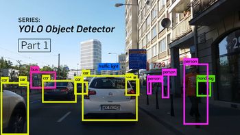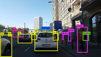
Image Credits: Karol Majek. Check out his YOLO v3 real time detection video here
This is Part 2 of the tutorial on implementing a YOLO v3 detector from scratch. In the last part, I explained how YOLO works, and in this part, we are going to implement the layers used by YOLO in PyTorch. In other words, this is the part where we create the building blocks of our model.
The code for this tutorial is designed to run on Python 3.5, and PyTorch 0.4. It can be found in it's entirety at this Github repo.
This tutorial is broken into 5 parts:
-
Part 2 (This one): Creating the layers of the network architecture
-
Part 4 : Objectness Confidence Thresholding and Non-maximum Suppression
Prerequisites
- Part 1 of the tutorial/knowledge of how YOLO works.
- Basic working knowledge of PyTorch, including how to create custom architectures with
nn.Module,nn.Sequentialandtorch.nn.parameterclasses.
I assume you have had some experiene with PyTorch before. If you're just starting out, I'd recommend you to play around with the framework a bit before returning to this post.
Getting Started
First create a directory where the code for detector will live.
Then, create a file darknet.py. Darknet is the name of the underlying architecture of YOLO. This file will contain the code that creates the YOLO network. We will supplement it with a file called util.py which will contain the code for various helper functions. Save both of these files in your detector folder. You can use git to keep track of the changes.
Configuration File
The official code (authored in C) uses a configuration file to build the network. The cfg file describes the layout of the network, block by block. If you're coming from a caffe background, it's equivalent to .protxt file used to describe the network.
We will use the official cfg file, released by the author to build our network. Download it from here and place it in a folder called cfg inside your detector directory. If you're on Linux, cd into your network directory and type:
mkdir cfg
cd cfg
wget https://raw.githubusercontent.com/pjreddie/darknet/master/cfg/yolov3.cfg
If you open the configuration file, you will see something like this.
[convolutional]
batch_normalize=1
filters=64
size=3
stride=2
pad=1
activation=leaky

[convolutional]
batch_normalize=1
filters=32
size=1
stride=1
pad=1
activation=leaky

[convolutional]
batch_normalize=1
filters=64
size=3
stride=1
pad=1
activation=leaky

[shortcut]
from=-3
activation=linear
We see 4 blocks above. Out of them, 3 describe convolutional layers, followed by a shortcut layer. A shortcut layer is a skip connection, like the one used in ResNet. There are 5 types of layers that are used in YOLO:
Convolutional
[convolutional]
batch_normalize=1
filters=64
size=3
stride=1
pad=1
activation=leaky
Shortcut
[shortcut]
from=-3
activation=linear
A shortcut layer is a skip connection, akin to the one used in ResNet. The from parameter is -3, which means the output of the shortcut layer is obtained by adding feature maps from the previous and the 3rd layer backwards from the shortcut layer.
Upsample
[upsample]
stride=2
Upsamples the feature map in the previous layer by a factor of stride using bilinear upsampling.
Route
[route]
layers = -4

[route]
layers = -1, 61
The route layer deserves a bit of explanation. It has an attribute layers which can have either one, or two values.
When layers attribute has only one value, it outputs the feature maps of the layer indexed by the value. In our example, it is -4, so the layer will output feature map from the 4th layer backwards from the Route layer.
When layers has two values, it returns the concatenated feature maps of the layers indexed by it's values. In our example it is -1, 61, and the layer will output feature maps from the previous layer (-1) and the 61st layer, concatenated along the depth dimension.
YOLO
[yolo]
mask = 0,1,2
anchors = 10,13,  16,30,  33,23,  30,61,  62,45,  59,119,  116,90,  156,198,  373,326
classes=80
num=9
jitter=.3
ignore_thresh = .5
truth_thresh = 1
random=1
YOLO layer corresponds to the Detection layer described in part 1. The anchors describes 9 anchors, but only the anchors which are indexed by attributes of the mask tag are used. Here, the value of mask is 0,1,2, which means the first, second and third anchors are used. This make sense since each cell of the detection layer predicts 3 boxes. In total, we have detection layers at 3 scales, making up for a total of 9 anchors.
Net
[net]
# Testing
batch=1
subdivisions=1
# Training
# batch=64
# subdivisions=16
width= 320
height = 320
channels=3
momentum=0.9
decay=0.0005
angle=0
saturation = 1.5
exposure = 1.5
hue=.1
There's another type of block called net in the cfg, but I wouldn't call it a layer as it only describes information about the network input and training parameters. It isn't used in the forward pass of YOLO. However, it does provide us with information like the network input size, which we use to adjust anchors in the forward pass.
Parsing the configuration file
Before we begin, add the necessary imports at the top of the darknet.py file.
from __future__ import division

import torch
import torch.nn as nn
import torch.nn.functional as F
from torch.autograd import Variable
import numpy as np
We define a function called parse_cfg, which takes the path of the configuration file as the input.
def parse_cfg(cfgfile):
    """
    Takes a configuration file

    Returns a list of blocks. Each blocks describes a block in the neural
    network to be built. Block is represented as a dictionary in the list

    """
The idea here is to parse the cfg, and store every block as a dict. The attributes of the blocks and their values are stored as key-value pairs in the dictionary. As we parse through the cfg, we keep appending these dicts, denoted by the variable block in our code, to a list blocks. Our function will return this block.
We begin by saving the content of the cfg file in a list of strings. The following code performs some preprocessing on this list.
file = open(cfgfile, 'r')
lines = file.read().split('\n')                        # store the lines in a list
lines = [x for x in lines if len(x) > 0]               # get read of the empty lines
lines = [x for x in lines if x[0] != '#']              # get rid of comments
lines = [x.rstrip().lstrip() for x in lines]           # get rid of fringe whitespaces
Then, we loop over the resultant list to get blocks.
block = {}
blocks = []

for line in lines:
    if line[0] == "[":               # This marks the start of a new block
        if len(block) != 0:          # If block is not empty, implies it is storing values of previous block.
            blocks.append(block)     # add it the blocks list
            block = {}               # re-init the block
        block["type"] = line[1:-1].rstrip()
    else:
        key,value = line.split("=")
        block[key.rstrip()] = value.lstrip()
blocks.append(block)

return blocks
Creating the building blocks
Now we are going to use the list returned by the above parse_cfg to construct PyTorch modules for the blocks present in the config file.
We have 5 types of layers in the list (mentioned above). PyTorch provides pre-built layers for types convolutional and upsample. We will have to write our own modules for the rest of the layers by extending the nn.Module class.
The create_modules function takes a list blocks returned by the parse_cfg function.
def create_modules(blocks):
    net_info = blocks[0]     #Captures the information about the input and pre-processing
    module_list = nn.ModuleList()
    prev_filters = 3
    output_filters = []
Before we iterate over list of blocks, we define a variable net_info to store information about the network.
nn.ModuleList
Our function will return a nn.ModuleList. This class is almost like a normal list containing nn.Module objects. However, when we add nn.ModuleList as a member of a nn.Module object (i.e. when we add modules to our network), all the parameters of nn.Module objects (modules) inside the nn.ModuleList are added as parameters of the nn.Module object (i.e. our network, which we are adding the nn.ModuleList as a member of) as well.
When we define a new convolutional layer, we must define the dimension of it's kernel. While the height and width of kernel is provided by the cfg file, the depth of the kernel is precisely the number of filters (or depth of the feature map) present in the previous layer. This means we need to keep track of number of filters in the layer on which the convolutional layer is being applied. We use the variable prev_filter to do this. We initialise this to 3, as the image has 3 filters corresponding to the RGB channels.
The route layer brings (possibly concatenated) feature maps from previous layers. If there's a convolutional layer right in front of a route layer, then the kernel is applied on the feature maps of previous layers, precisely the ones the route layer brings. Therefore, we need to keep a track of the number of filters in not only the previous layer, but each one of the preceding layers. As we iterate, we append the number of output filters of each block to the list output_filters.
Now, the idea is to iterate over the list of blocks, and create a PyTorch module for each block as we go.
    for index, x in enumerate(blocks[1:]):
        module = nn.Sequential()

        #check the type of block
        #create a new module for the block
        #append to module_list
nn.Sequential class is used to sequentially execute a number of nn.Module objects. If you look at the cfg, you will realize a block may contain more than one layer. For example, a block of type convolutional has a batch norm layer as well as leaky ReLU activation layer in addition to a convolutional layer. We string together these layers using the nn.Sequential and it's the add_module function. For example, this is how we create the convolutional and the upsample layers.
        if (x["type"] == "convolutional"):
            #Get the info about the layer
            activation = x["activation"]
            try:
                batch_normalize = int(x["batch_normalize"])
                bias = False
            except:
                batch_normalize = 0
                bias = True

            filters= int(x["filters"])
            padding = int(x["pad"])
            kernel_size = int(x["size"])
            stride = int(x["stride"])

            if padding:
                pad = (kernel_size - 1) // 2
            else:
                pad = 0

            #Add the convolutional layer
            conv = nn.Conv2d(prev_filters, filters, kernel_size, stride, pad, bias = bias)
            module.add_module("conv_{0}".format(index), conv)

            #Add the Batch Norm Layer
            if batch_normalize:
                bn = nn.BatchNorm2d(filters)
                module.add_module("batch_norm_{0}".format(index), bn)

            #Check the activation.
            #It is either Linear or a Leaky ReLU for YOLO
            if activation == "leaky":
                activn = nn.LeakyReLU(0.1, inplace = True)
                module.add_module("leaky_{0}".format(index), activn)

        #If it's an upsampling layer
        #We use Bilinear2dUpsampling
        elif (x["type"] == "upsample"):
            stride = int(x["stride"])
            upsample = nn.Upsample(scale_factor = 2, mode = "bilinear")
            module.add_module("upsample_{}".format(index), upsample)
Route Layer / Shortcut Layers
Next, we write the code for creating the Route and the Shortcut Layers.
        #If it is a route layer
        elif (x["type"] == "route"):
            x["layers"] = x["layers"].split(',')
            #Start  of a route
            start = int(x["layers"][0])
            #end, if there exists one.
            try:
                end = int(x["layers"][1])
            except:
                end = 0
            #Positive anotation
            if start > 0:
                start = start - index
            if end > 0:
                end = end - index
            route = EmptyLayer()
            module.add_module("route_{0}".format(index), route)
            if end < 0:
                filters = output_filters[index + start] + output_filters[index + end]
            else:
                filters= output_filters[index + start]

        #shortcut corresponds to skip connection
        elif x["type"] == "shortcut":
            shortcut = EmptyLayer()
            module.add_module("shortcut_{}".format(index), shortcut)
The code for creating the Route Layer deserves a fair bit of explanation. At first, we extract the the value of the layers attribute, cast it into an integer and store it in a list.
Then we have a new layer called EmptyLayer which, as the name suggests is just an empty layer.
route = EmptyLayer()
It is defined as.
class EmptyLayer(nn.Module):
    def __init__(self):
        super(EmptyLayer, self).__init__()
Wait, an empty layer?
Now, an empty layer might seem weird given it does nothing. The Route Layer, just like any other layer performs an operation (bringing forward previous layer / concatenation). In PyTorch, when we define a new layer, we subclass nn.Module and write the operation the layer performs in the forward function of the nn.Module object.
For designing a layer for the Route block, we will have to build a nn.Module object that is initialized with values of the attribute layers as it's member(s). Then, we can write the code to concatenate/bring forward the feature maps in the forward function. Finally, we then execute this layer in th forward function of our network.
But given the code of concatenation is fairly short and simple (calling torch.cat on feature maps), designing a layer as above will lead to unnecessary abstraction that just increases boiler plate code. Instead, what we can do is put a dummy layer in place of a proposed route layer, and then perform the concatenation directly in the forward function of the nn.Module object representing darknet. (If the last line doesn't make a lot of sense to you, I suggest you to read how nn.Module class is used in PyTorch. Link at the bottom)
The convolutional layer just in front of a route layer applies it's kernel to (possibly concatenated) feature maps from a previous layers. The following code updates the filters variable to hold the number of filters outputted by a route layer.
if end < 0:
    #If we are concatenating maps
    filters = output_filters[index + start] + output_filters[index + end]
else:
    filters= output_filters[index + start]
The shortcut layer also makes use of an empty layer, for it also performs a very simple operation (addition). There is no need to update update the filters variable as it merely adds a feature maps of a previous layer to those of layer just behind.
YOLO Layer
Finally, we write the code for creating the the YOLO layer.
        #Yolo is the detection layer
        elif x["type"] == "yolo":
            mask = x["mask"].split(",")
            mask = [int(x) for x in mask]

            anchors = x["anchors"].split(",")
            anchors = [int(a) for a in anchors]
            anchors = [(anchors[i], anchors[i+1]) for i in range(0, len(anchors),2)]
            anchors = [anchors[i] for i in mask]

            detection = DetectionLayer(anchors)
            module.add_module("Detection_{}".format(index), detection)
We define a new layer DetectionLayer that holds the anchors used to detect bounding boxes.
The detection layer is defined as
class DetectionLayer(nn.Module):
    def __init__(self, anchors):
        super(DetectionLayer, self).__init__()
        self.anchors = anchors
At the end of the loop, we do some bookkeeping.
        module_list.append(module)
        prev_filters = filters
        output_filters.append(filters)
That concludes the body of the loop. At the end of the function create_modules, we return a tuple containing the net_info, and module_list.
return (net_info, module_list)
Testing the code
You can test your code by typing the following lines at the end of darknet.py and running the file.
blocks = parse_cfg("cfg/yolov3.cfg")
print(create_modules(blocks))
You will see a long list, (exactly containing 106 items), the elements of which will look like
.
.

  (9): Sequential(
     (conv_9): Conv2d (128, 64, kernel_size=(1, 1), stride=(1, 1), bias=False)
     (batch_norm_9): BatchNorm2d(64, eps=1e-05, momentum=0.1, affine=True)
     (leaky_9): LeakyReLU(0.1, inplace)
   )
   (10): Sequential(
     (conv_10): Conv2d (64, 128, kernel_size=(3, 3), stride=(1, 1), padding=(1, 1), bias=False)
     (batch_norm_10): BatchNorm2d(128, eps=1e-05, momentum=0.1, affine=True)
     (leaky_10): LeakyReLU(0.1, inplace)
   )
   (11): Sequential(
     (shortcut_11): EmptyLayer(
     )
   )
.
.
.
That's it for this part. In this next part, we will assemble the building blocks that we've created to produce output from an image.
Further Reading
Ayoosh Kathuria is currently an intern at the Defense Research and Development Organization, India, where he is working on improving object detection in grainy videos. When he's not working, he's either sleeping or playing pink floyd on his guitar. You can connect with him on LinkedIn or look at more of what he does at GitHub