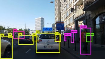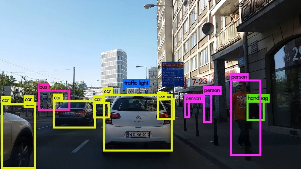
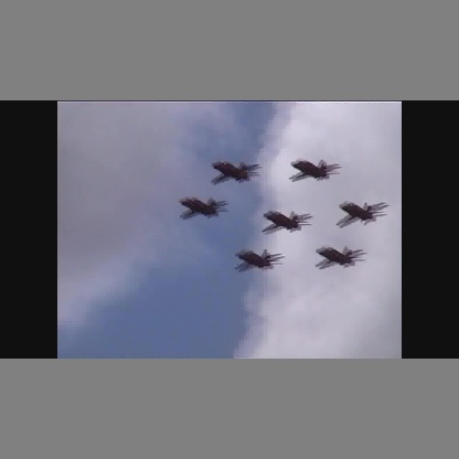
Image Credits: Karol Majek. Check out his YOLO v3 real time detection video here
This is Part 5 of the tutorial on implementing a YOLO v3 detector from scratch. In the last part, we implemented a function to transform the output of the network into detection predictions. With a working detector at hand, all that's left is to create input and output pipelines.
The code for this tutorial is designed to run on Python 3.5, and PyTorch 0.4. It can be found in it's entirety at this Github repo.
This tutorial is broken into 5 parts:
-
Part 4 : Confidence Thresholding and Non-maximum Suppression
-
Part 5 (This one): Designing the input and the output pipelines
Prerequisites
- Part 1-4 of the tutorial.
- Basic working knowledge of PyTorch, including how to create custom architectures with nn.Module, nn.Sequential and torch.nn.parameter classes.
- Basic knowledge of OpenCV
EDIT: If you've visited this post earlier than 30/03/2018, the way we resized an arbitarily sized image to Darknet's input size was by simply rescaling the dimensions. However, in the original implementation, an image is resized keeping the aspect ratio intact, and padding the left-out portions. For example, if we were to resize a 1900 x 1280 image to 416 x 415, the resized image would look like this.
This difference in preparing the input caused the earlier implementation to have marginally inferior performance to the original. However, the post has been updated to incorporate the resizing metho followed in the original implementation
In this part we will build the input and the output pipelines of our detector. This involves the reading images off the disk, making a prediction, using the prediction to draw bounding boxes on images, and then saving them to the disk. We will also cover how to have the detector work in real time on a camera feed or a video. We will introduce some command line flags to allow some experimentation with various hyperparamters of the network. So let's begin.
Note: You will need to install OpenCV 3 for this part.
Create a file detector.py in tour detector file. Add neccasary imports at top of it.
from __future__ import division
import time
import torch
import torch.nn as nn
from torch.autograd import Variable
import numpy as np
import cv2
from util import *
import argparse
import os
import os.path as osp
from darknet import Darknet
import pickle as pkl
import pandas as pd
import random
Creating Command Line Arguments
Since detector.py is the file that we will execute to run our detector, it's nice to have command line arguments we can pass to it. I've used python's ArgParse module to do that.
def arg_parse():
    """
    Parse arguements to the detect module

    """

    parser = argparse.ArgumentParser(description='YOLO v3 Detection Module')

    parser.add_argument("--images", dest = 'images', help =
                        "Image / Directory containing images to perform detection upon",
                        default = "imgs", type = str)
    parser.add_argument("--det", dest = 'det', help =
                        "Image / Directory to store detections to",
                        default = "det", type = str)
    parser.add_argument("--bs", dest = "bs", help = "Batch size", default = 1)
    parser.add_argument("--confidence", dest = "confidence", help = "Object Confidence to filter predictions", default = 0.5)
    parser.add_argument("--nms_thresh", dest = "nms_thresh", help = "NMS Threshhold", default = 0.4)
    parser.add_argument("--cfg", dest = 'cfgfile', help =
                        "Config file",
                        default = "cfg/yolov3.cfg", type = str)
    parser.add_argument("--weights", dest = 'weightsfile', help =
                        "weightsfile",
                        default = "yolov3.weights", type = str)
    parser.add_argument("--reso", dest = 'reso', help =
                        "Input resolution of the network. Increase to increase accuracy. Decrease to increase speed",
                        default = "416", type = str)

    return parser.parse_args()

args = arg_parse()
images = args.images
batch_size = int(args.bs)
confidence = float(args.confidence)
nms_thesh = float(args.nms_thresh)
start = 0
CUDA = torch.cuda.is_available()
Amongst these, important flags are images (used to specify the input image or directory of images), det (Directory to save detections to), reso (Input image's resolution, can be used for speed - accuracy tradeoff), cfg (alternative configuration file) and weightfile.
Loading the Network
Download the file coco.names from here, a file that contains the names of the objects in the COCO dataset. Create a folder data in your detector directory. Equivalently, if you're on linux you can type.
mkdir data
cd data
wget https://raw.githubusercontent.com/ayooshkathuria/YOLO_v3_tutorial_from_scratch/master/data/coco.names
Then, we load the class file in our program.
num_classes = 80    #For COCO
classes = load_classes("data/coco.names")
load_classes is a function defined in util.py that returns a dictionary which maps the index of every class to a string of it's name.
def load_classes(namesfile):
    fp = open(namesfile, "r")
    names = fp.read().split("\n")[:-1]
    return names
Initialize the network and load weights.
#Set up the neural network
print("Loading network.....")
model = Darknet(args.cfgfile)
model.load_weights(args.weightsfile)
print("Network successfully loaded")

model.net_info["height"] = args.reso
inp_dim = int(model.net_info["height"])
assert inp_dim % 32 == 0
assert inp_dim > 32

#If there's a GPU availible, put the model on GPU
if CUDA:
    model.cuda()

#Set the model in evaluation mode
model.eval()
Read the Input images
Read the image from the disk, or the images from a directory. The paths of the image/images are stored in a list called imlist.
read_dir = time.time()
#Detection phase
try:
    imlist = [osp.join(osp.realpath('.'), images, img) for img in os.listdir(images)]
except NotADirectoryError:
    imlist = []
    imlist.append(osp.join(osp.realpath('.'), images))
except FileNotFoundError:
    print ("No file or directory with the name {}".format(images))
    exit()
read_dir is a checkpoint used to measure time. (We will encounter several of these)
If the directory to save the detections, defined by the det flag, doesn't exist, create it.
if not os.path.exists(args.det):
    os.makedirs(args.det)
We will use OpenCV to load the images.
load_batch = time.time()
loaded_ims = [cv2.imread(x) for x in imlist]
load_batch is again a checkpoint.
OpenCV loads an image as an numpy array, with BGR as the order of the color channels. PyTorch's image input format is (Batches x Channels x Height x Width), with the channel order being RGB. Therefore, we write the function prep_image in util.py to transform the numpy array into PyTorch's input format.
Before we can write this function, we must write a function letterbox_image that resizes our image, keeping the aspect ratio consistent, and padding the left out areas with the color (128,128,128)
def letterbox_image(img, inp_dim):
    '''resize image with unchanged aspect ratio using padding'''
    img_w, img_h = img.shape[1], img.shape[0]
    w, h = inp_dim
    new_w = int(img_w * min(w/img_w, h/img_h))
    new_h = int(img_h * min(w/img_w, h/img_h))
    resized_image = cv2.resize(img, (new_w,new_h), interpolation = cv2.INTER_CUBIC)

    canvas = np.full((inp_dim[1], inp_dim[0], 3), 128)

    canvas[(h-new_h)//2:(h-new_h)//2 + new_h,(w-new_w)//2:(w-new_w)//2 + new_w,  :] = resized_image

    return canvas
Now, we write the function that takes a OpenCV images and converts it to the input of our network.
def prep_image(img, inp_dim):
    """
    Prepare image for inputting to the neural network.

    Returns a Variable
    """

    img = cv2.resize(img, (inp_dim, inp_dim))
    img = img[:,:,::-1].transpose((2,0,1)).copy()
    img = torch.from_numpy(img).float().div(255.0).unsqueeze(0)
    return img
In addition to the transformed image, we also maintain a list of original images, and im_dim_list, a list containing the dimensions of the original images.
#PyTorch Variables for images
im_batches = list(map(prep_image, loaded_ims, [inp_dim for x in range(len(imlist))]))

#List containing dimensions of original images
im_dim_list = [(x.shape[1], x.shape[0]) for x in loaded_ims]
im_dim_list = torch.FloatTensor(im_dim_list).repeat(1,2)

if CUDA:
    im_dim_list = im_dim_list.cuda()
Create the Batches
leftover = 0
if (len(im_dim_list) % batch_size):
   leftover = 1

if batch_size != 1:
   num_batches = len(imlist) // batch_size + leftover
   im_batches = [torch.cat((im_batches[i*batch_size : min((i +  1)*batch_size,
                       len(im_batches))]))  for i in range(num_batches)]
The Detection Loop
We iterate over the batches, generate the prediction, and concatenate the prediction tensors (of shape, D x 8, the output of write_results function) of all the images we have to perform detections upon.
For each batch, we measure the time taken for detection as the time spent between taking the input, and producing the output of the write_results function. In the output returned by write_prediction, one of the attributes was the index of the image in batch. We transform that particular attribute in such a way that it now represents the index of the image in imlist, the list containing addresses of all images.
After that, we print time taken for each detection as well as the object detected in each image.
If the output of the write_results function for batch is an int(0), meaning there is no detection, we use continue to skip the rest loop.
write = 0
start_det_loop = time.time()
for i, batch in enumerate(im_batches):
    #load the image
    start = time.time()
    if CUDA:
        batch = batch.cuda()

    prediction = model(Variable(batch, volatile = True), CUDA)

    prediction = write_results(prediction, confidence, num_classes, nms_conf = nms_thesh)

    end = time.time()

    if type(prediction) == int:

        for im_num, image in enumerate(imlist[i*batch_size: min((i +  1)*batch_size, len(imlist))]):
            im_id = i*batch_size + im_num
            print("{0:20s} predicted in {1:6.3f} seconds".format(image.split("/")[-1], (end - start)/batch_size))
            print("{0:20s} {1:s}".format("Objects Detected:", ""))
            print("----------------------------------------------------------")
        continue

    prediction[:,0] += i*batch_size    #transform the atribute from index in batch to index in imlist

    if not write:                      #If we have't initialised output
        output = prediction
        write = 1
    else:
        output = torch.cat((output,prediction))

    for im_num, image in enumerate(imlist[i*batch_size: min((i +  1)*batch_size, len(imlist))]):
        im_id = i*batch_size + im_num
        objs = [classes[int(x[-1])] for x in output if int(x[0]) == im_id]
        print("{0:20s} predicted in {1:6.3f} seconds".format(image.split("/")[-1], (end - start)/batch_size))
        print("{0:20s} {1:s}".format("Objects Detected:", " ".join(objs)))
        print("----------------------------------------------------------")

    if CUDA:
        torch.cuda.synchronize()
The line torch.cuda.synchronize makes sure that CUDA kernel is synchronized with the CPU. Otherwise, CUDA kernel returns the control to CPU as soon as the GPU job is queued and well before the GPU job is completed (Asynchronous calling). This might lead to a misleading time if end = time.time() gets printed before the GPU job is actually over.
Now, we have the detections of all images in our Tensor Output. Let us draw the bounding boxes on images.
Drawing bounding boxes on images
We use a try-catch block to check whether there has been a single detection has been made or not. If that's not the case, exit the program.
try:
    output
except NameError:
    print ("No detections were made")
    exit()
Before we draw the bounding boxes, the predictions contained in our output tensor conform to the input size of the network, and not the original sizes of the images. So, before we can draw the bounding boxes, let us transform the corner attributes of each bounding box, to the original dimensions of images.
Before we draw the bounding boxes, the predictions contained in our output tensor are predictions on the padded image, and not the original image. Merely, re-scaling them to the dimensions of the input image won't work here. We first need to transform the co-ordinates of the boxes to be measured with respect to boundaries of the area on the padded image that contains the original image.
im_dim_list = torch.index_select(im_dim_list, 0, output[:,0].long())

scaling_factor = torch.min(inp_dim/im_dim_list,1)[0].view(-1,1)


output[:,[1,3]] -= (inp_dim - scaling_factor*im_dim_list[:,0].view(-1,1))/2
output[:,[2,4]] -= (inp_dim - scaling_factor*im_dim_list[:,1].view(-1,1))/2
Now, our co-ordinates conform to dimensions of our image on the padded area. However, in the function letterbox_image, we had resized both the dimensions of our image by a scaling factor (remember both dimensions were divided with a common factor to maintain aspect ratio). We now undo this rescaling to get the co-ordinates of the bounding box on the original image.
output[:,1:5] /= scaling_factor
Let us now clip any bounding boxes that may have boundaries outside the image to the edges of our image.
for i in range(output.shape[0]):
    output[i, [1,3]] = torch.clamp(output[i, [1,3]], 0.0, im_dim_list[i,0])
    output[i, [2,4]] = torch.clamp(output[i, [2,4]], 0.0, im_dim_list[i,1])
If there are too many bounding boxes in the image, drawing them all in one color may not be such a nice idea. Download this file to your detector folder. This is a pickled file that contains many colors to randomly choose from.
class_load = time.time()
colors = pkl.load(open("pallete", "rb"))
Now let us write a function to draw the boxes.
draw = time.time()

def write(x, results, color):
    c1 = tuple(x[1:3].int())
    c2 = tuple(x[3:5].int())
    img = results[int(x[0])]
    cls = int(x[-1])
    label = "{0}".format(classes[cls])
    cv2.rectangle(img, c1, c2,color, 1)
    t_size = cv2.getTextSize(label, cv2.FONT_HERSHEY_PLAIN, 1 , 1)[0]
    c2 = c1[0] + t_size[0] + 3, c1[1] + t_size[1] + 4
    cv2.rectangle(img, c1, c2,color, -1)
    cv2.putText(img, label, (c1[0], c1[1] + t_size[1] + 4), cv2.FONT_HERSHEY_PLAIN, 1, [225,255,255], 1);
    return img
The function above draws a rectangle with a color of a random choice from colors. It also creates a filled rectangle on the top left corner of the bounding box, and writes the class of the object detected across the filled rectangle. -1 argument of the cv2.rectangle function is used for creating a filled rectangle.
We define write function locally so that it can access the colors list. We could have also included colors as an argument, but that would have allowed us to use only one color per image, which defeats the purpose of what we want to do.
Once we've defined this function, let us now draw the bounding boxes on images.
list(map(lambda x: write(x, loaded_ims), output))
The above snippet modifies the images inside loaded_ims inplace.
Each image is saved by prefixing the "det_" in front of the image name. We create a list of addresses, to which we will save the our detection images to.
det_names = pd.Series(imlist).apply(lambda x: "{}/det_{}".format(args.det,x.split("/")[-1]))
Finally, write the images with detections to the address in det_names.
list(map(cv2.imwrite, det_names, loaded_ims))
end = time.time()
Printing Time Summary
At the end of our detector we will print a summary containing which part of the code took how long to execute. This is useful when we have to compare how different hyperparameters effect the speed of the detector. Hyperparameters such as batch size, objectness confidence and NMS threshold, (passed with bs, confidence, nms_thresh flags respectively) can be set while executing the script detection.py on the command line.
print("SUMMARY")
print("----------------------------------------------------------")
print("{:25s}: {}".format("Task", "Time Taken (in seconds)"))
print()
print("{:25s}: {:2.3f}".format("Reading addresses", load_batch - read_dir))
print("{:25s}: {:2.3f}".format("Loading batch", start_det_loop - load_batch))
print("{:25s}: {:2.3f}".format("Detection (" + str(len(imlist)) +  " images)", output_recast - start_det_loop))
print("{:25s}: {:2.3f}".format("Output Processing", class_load - output_recast))
print("{:25s}: {:2.3f}".format("Drawing Boxes", end - draw))
print("{:25s}: {:2.3f}".format("Average time_per_img", (end - load_batch)/len(imlist)))
print("----------------------------------------------------------")


torch.cuda.empty_cache()
Testing The Object Detector
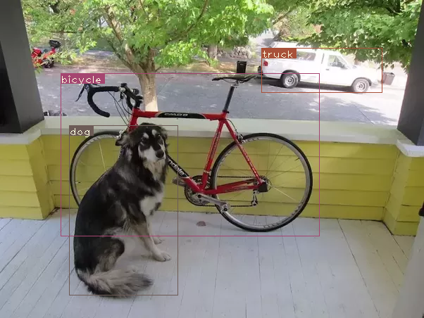
For example, running on terminal,
python detect.py --images dog-cycle-car.png --det det
produces the output
The following code is run on CPU. Expect detection times to be much much faster on GPU. It's around 0.1 sec / image on a Tesla K80.
Loading network.....
Network successfully loaded
dog-cycle-car.png    predicted in  2.456 seconds
Objects Detected:    bicycle truck dog
----------------------------------------------------------
SUMMARY
----------------------------------------------------------
Task                     : Time Taken (in seconds)

Reading addresses        : 0.002
Loading batch            : 0.120
Detection (1 images)     : 2.457
Output Processing        : 0.002
Drawing Boxes            : 0.076
Average time_per_img     : 2.657
----------------------------------------------------------
An image with name det_dog-cycle-car.png is saved in the det directory.
Running the Detector on Video/Webcam
In order to run the detector on the video or webcam, the code remains almost the same, except we don't have to iterate over batches, but frames of a video.
The code for running the detector on the video can be found in the file video.py in the github repository. The code is very similar to that of detect.py except for a few changes.
First, we open the video / camera feed in OpenCV.
videofile = "video.avi" #or path to the video file.

cap = cv2.VideoCapture(videofile)

#cap = cv2.VideoCapture(0)  for webcam

assert cap.isOpened(), 'Cannot capture source'

frames = 0
The we iterate over the frames in a similar fashion to the way we iterated over images.
A lot of code has been simplified over many places because we no longer have to deal with batches, but only one image at a time. This is because only one frame can come at a time. This includes using a tuple in place of a tensor for im_dim_list and a minute change in the write function.
Every iteration, we keep a track of the number of frames captured in a variable called frames. We then divide this number by the time elapsed since the first frame to print the FPS of the video.
Instead for writing the detection images to disk using cv2.imwrite, we use cv2.imshow to display the frame with bounding box drawn on it. If the user presses the Q button, it causes the code to break the loop, and the video ends.
frames = 0
start = time.time()

while cap.isOpened():
    ret, frame = cap.read()

    if ret:
        img = prep_image(frame, inp_dim)
#        cv2.imshow("a", frame)
        im_dim = frame.shape[1], frame.shape[0]
        im_dim = torch.FloatTensor(im_dim).repeat(1,2)

        if CUDA:
            im_dim = im_dim.cuda()
            img = img.cuda()

        output = model(Variable(img, volatile = True), CUDA)
        output = write_results(output, confidence, num_classes, nms_conf = nms_thesh)


        if type(output) == int:
            frames += 1
            print("FPS of the video is {:5.4f}".format( frames / (time.time() - start)))
            cv2.imshow("frame", frame)
            key = cv2.waitKey(1)
            if key & 0xFF == ord('q'):
                break
            continue
        output[:,1:5] = torch.clamp(output[:,1:5], 0.0, float(inp_dim))

        im_dim = im_dim.repeat(output.size(0), 1)/inp_dim
        output[:,1:5] *= im_dim

        classes = load_classes('data/coco.names')
        colors = pkl.load(open("pallete", "rb"))

        list(map(lambda x: write(x, frame), output))

        cv2.imshow("frame", frame)
        key = cv2.waitKey(1)
        if key & 0xFF == ord('q'):
            break
        frames += 1
        print(time.time() - start)
        print("FPS of the video is {:5.2f}".format( frames / (time.time() - start)))
    else:
        break
Conclusion
In this series of tutorials, we have implemented an object detector from scratch, and cheers for reaching this far. I still think being able to churn out efficient code is one of the most underrated skills a deep learning practitioner can have. However revolutionary your idea you maybe, it's of no use unless you can test it. For that, you need to have strong coding skills.
I've also learned that the the best way to learn about any topic in deep learning is to implement code. It forces you to glance over the minute yet fundamental subtleties of a topic that you may miss out on when you're reading a paper. I hope this tutorial series has served as an exercise in honing your skills as a deep learning practitioner.
Further Reading
Ayoosh Kathuria is currently an intern at the Defense Research and Development Organization, India, where he is working on improving object detection in grainy videos. When he's not working, he's either sleeping or playing pink floyd on his guitar. You can connect with him on LinkedIn or look at more of what he does at GitHub