In this article, we will discuss how to use PyTorch to build custom neural network architectures, and how to configure your training loop. We will implement a ResNet to classify images from the CIFAR-10 Dataset.

Before, we begin, let me say that the purpose of this tutorial is not to achieve the best possible accuracy on the task, but to show you how to use PyTorch.

Let me also remind you that this is the Part 2 of the our tutorial series on PyTorch. Reading the first part, though not necessary for this article, is highly recommended.

1. Understanding Graphs, Automatic Differentiation and Autograd
2. Building Your First Neural Network
3. Going Deep with PyTorch
4. Memory Management and Using Multiple GPUs
5. Understanding Hooks

You can get all the code in this post, (and other posts as well) in the Github repo here.

In this post, we will cover

1. How to build neural networks using nn.Module class
2. How to build custom data input pipelines with data augmentation using Dataset and Dataloader classes.
3. How to configure your learning rate with different learning rate schedules
4. Training a Resnet bases image classifier to classify images from the CIFAR-10 dataset.

Prerequisites

1. Chain rule
2. Basic Understanding of Deep Learning
3. PyTorch 1.0
4. Part 1 of this tutorial

You can get all the code in this post, (and other posts as well) in the Github repo here.

A Simple Neural Network

In this tutorial, we will be implementing a very simple neural network.  

Building the Network

The torch.nn  module is the cornerstone of designing neural networks in PyTorch. This class can be used to implement a layer like a fully connected layer, a convolutional layer, a pooling layer, an activation function, and also an entire neural network by instantiating a torch.nn.Module object. (From now on, I'll refer to it as merely nn.module)

Multiple nn.Module objects can be strung together to form a bigger nn.Module object, which is how we can implement a neural network using many layers. In fact, nn.Module can be used to represent an arbitrary function f in PyTorch.

The nn.Module class has two methods that you have to override.

1. __init__ function. This function is invoked when you create an instance of the nn.Module. Here you will define the various parameters of a layer such as filters, kernel size for a convolutional layer, dropout probability for the dropout layer.
2. forward function. This is where you define how your output is computed. This function doesn't need to be explicitly called, and can be run by just calling the nn.Module instance like a function with the input as it's argument.

# Very simple layer that just multiplies the input by a number
class MyLayer(nn.Module):
  def __init__(self, param):
    super().__init__()
    self.param = param 
  
  def forward(self, x):
    return x * self.param
  
myLayerObject = MyLayer(5)
output = myLayerObject(torch.Tensor([5, 4, 3]) )    #calling forward inexplicitly 
print(output)

Another widely used and important class is the nn.Sequential class.  When initiating this class we can pass a list of nn.Module objects in a particular sequence. The object returned by nn.Sequential is itself a nn.Module object. When this object is run with an input, it sequentially runs the input through all the nn.Module object we passed to it, in the very same order as we passed them.

combinedNetwork = nn.Sequential(MyLayer(5), MyLayer(10))

output = combinedNetwork([3,4])

#equivalent to..
# out = MyLayer(5)([3,4])
# out = MyLayer(10)(out)

Let us now start implementing our classification network. We will make use of convolutional and pooling layers, as well as a custom implemented residual block.

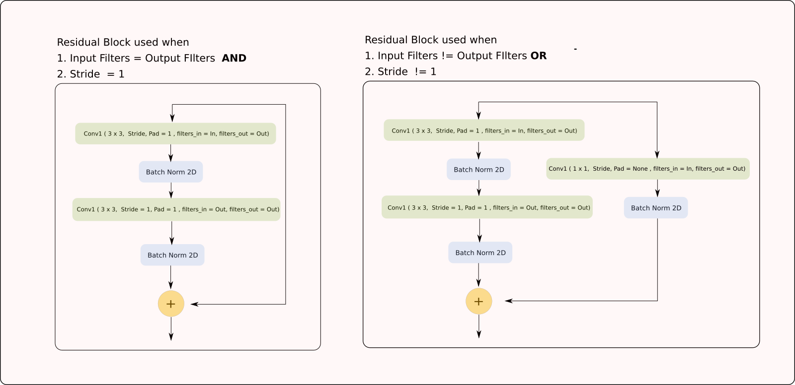
While PyTorch provided many layers out of the box with it's torch.nn module, we will have to implement the residual block ourselves. Before implementing the neural network, we implement the ResNet Block.

class ResidualBlock(nn.Module):
    def __init__(self, in_channels, out_channels, stride=1):
        super(ResidualBlock, self).__init__()
        
        # Conv Layer 1
        self.conv1 = nn.Conv2d(
            in_channels=in_channels, out_channels=out_channels,
            kernel_size=(3, 3), stride=stride, padding=1, bias=False
        )
        self.bn1 = nn.BatchNorm2d(out_channels)
        
        # Conv Layer 2
        self.conv2 = nn.Conv2d(
            in_channels=out_channels, out_channels=out_channels,
            kernel_size=(3, 3), stride=1, padding=1, bias=False
        )
        self.bn2 = nn.BatchNorm2d(out_channels)
    
        # Shortcut connection to downsample residual
        # In case the output dimensions of the residual block is not the same 
        # as it's input, have a convolutional layer downsample the layer 
        # being bought forward by approporate striding and filters
        self.shortcut = nn.Sequential()
        if stride != 1 or in_channels != out_channels:
            self.shortcut = nn.Sequential(
                nn.Conv2d(
                    in_channels=in_channels, out_channels=out_channels,
                    kernel_size=(1, 1), stride=stride, bias=False
                ),
                nn.BatchNorm2d(out_channels)
            )

    def forward(self, x):
        out = nn.ReLU()(self.bn1(self.conv1(x)))
        out = self.bn2(self.conv2(out))
        out += self.shortcut(x)
        out = nn.ReLU()(out)
        return out

As you see, we define the layers, or the components of our network in the __init__ function. In the forward function, how are we going to string together these components to compute the output from our input.

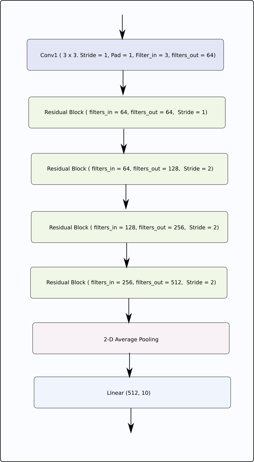
Now, we can define our full network.

class ResNet(nn.Module):
    def __init__(self, num_classes=10):
        super(ResNet, self).__init__()
        
        # Initial input conv
        self.conv1 = nn.Conv2d(
            in_channels=3, out_channels=64, kernel_size=(3, 3),
            stride=1, padding=1, bias=False
        )

        self.bn1 = nn.BatchNorm2d(64)
        
        # Create blocks
        self.block1 = self._create_block(64, 64, stride=1)
        self.block2 = self._create_block(64, 128, stride=2)
        self.block3 = self._create_block(128, 256, stride=2)
        self.block4 = self._create_block(256, 512, stride=2)
        self.linear = nn.Linear(512, num_classes)
    
    # A block is just two residual blocks for ResNet18
    def _create_block(self, in_channels, out_channels, stride):
        return nn.Sequential(
            ResidualBlock(in_channels, out_channels, stride),
            ResidualBlock(out_channels, out_channels, 1)
        )

    def forward(self, x):
	# Output of one layer becomes input to the next
        out = nn.ReLU()(self.bn1(self.conv1(x)))
        out = self.stage1(out)
        out = self.stage2(out)
        out = self.stage3(out)
        out = self.stage4(out)
        out = nn.AvgPool2d(4)(out)
        out = out.view(out.size(0), -1)
        out = self.linear(out)
        return out

Input Format

Now that we have our network object, we turn our focus to the input. We come across different types of input while working with Deep Learning. Images, audio or high dimensional structural data.

The kind of data we are dealing with will dictate what input we use. Generally, in PyTorch, you will realise that batch is always the first dimension. Since we are dealing with Images here, I will describe the input format required by images.  

The input format for images is [B C H W]. Where B is the batch size, C are the channels, H is the height and W is the width.

The output of our neural network is gibberish right now since we have used random weights. Let us now train our network.

Loading The Data

Let us now load the data. We will be making the use of torch.utils.data.Dataset and torch.utils.data.Dataloader class for this.

We first start by downloading the CIFAR-10 dataset in the same directory as our code file.

Fire up the terminal, cd to your code directory and run the following commands.

wget http://pjreddie.com/media/files/cifar.tgz
tar xzf cifar.tgz

You might need to use curl if you're on macOS or manually download it if you're on windows.

We now read the labels of the classes present in the CIFAR dataset.

data_dir = "cifar/train/"

with open("cifar/labels.txt") as label_file:
    labels = label_file.read().split()
    label_mapping = dict(zip(labels, list(range(len(labels)))))
     
    

We will be reading images using PIL library. Before we write the functionality to load our data, we write a preprocessing function that does the following things.

1. Randomly horizontally the image with a probability of 0.5
2. Normalise the image with mean and standard deviation of CIFAR dataset
3. Reshape it from W  H  C to C  H  W.

def preprocess(image):
    image = np.array(image)
    
    if random.random() > 0.5:
        image = image[::-1,:,:]
    
    cifar_mean = np.array([0.4914, 0.4822, 0.4465]).reshape(1,1,-1)
    cifar_std  = np.array([0.2023, 0.1994, 0.2010]).reshape(1,1,-1)
    image = (image - cifar_mean) / cifar_std
    
    image = image.transpose(2,1,0)
    return image
    

Normally, there are two classes PyTorch provides you in relation to build input pipelines to load data.

1. torch.data.utils.dataset, which we will just refer as the dataset class now.
2. torch.data.utils.dataloader , which we will just refer as the dataloader class now.

torch.utils.data.dataset

dataset is a class that loads the data and returns a generator so that you iterate over it. It also lets you incorporate data augmentation techniques into the input Pipeline.

If you want to create a dataset object for your data, you need to overload three functions.

1. __init__ function. Here, you define things related to your dataset here. Most importantly, the location of your data. You can also define various data augmentations you want to apply.
2. __len__ function. Here, you just return the length of the dataset.
3. __getitem__ function. The function takes as an argument an index i and returns a data example. This function would be called every iteration during our training loop with a different i by the dataset object.

Here is a implementation of our dataset object for the CIFAR dataset.

class Cifar10Dataset(torch.utils.data.Dataset):
    def __init__(self, data_dir, data_size = 0, transforms = None):
        files = os.listdir(data_dir)
        files = [os.path.join(data_dir,x) for x in files]
        
        
        if data_size < 0 or data_size > len(files):
            assert("Data size should be between 0 to number of files in the dataset")
        
        if data_size == 0:
            data_size = len(files)
        
        self.data_size = data_size
        self.files = random.sample(files, self.data_size)
        self.transforms = transforms
        
    def __len__(self):
        return self.data_size
    
    def __getitem__(self, idx):
        image_address = self.files[idx]
        image = Image.open(image_address)
        image = preprocess(image)
        label_name = image_address[:-4].split("_")[-1]
        label = label_mapping[label_name]
        
        image = image.astype(np.float32)
        
        if self.transforms:
            image = self.transforms(image)

        return image, label
        

We also use the __getitem__ function to extract the label for an image encoded in its file name.  

Dataset class allows us to incorporate the lazy data loading principle. This means instead of loading all data at once into the memory (which could be done by loading all the images in memory in the __init__ function rather than just addresses), it only loads a data example whenever it is needed (when __getitem__ is called).

When you create an object of the Dataset class, you basically can iterate over the object as you would over any python iterable. Each iteration, __getitem__ with the incremented index i as its input argument.

Data Augmentations

I've passed a transforms  argument in the __init__ function as well. This can be any python function that does data augmentation. While you can do the data augmentation right inside your preprocess code, doing it inside the __getitem__ is just a matter of taste.

Here, we can also add data augmentation. These data augmentations can be implemented as either functions or classes. You just have to make sure that you are able to apply them to your desired outcome in the __getitem__  function.

We have a plethora of data augmentation libraries that can be used to augment data.

For our case, torchvision library provides a lot of pre-built transforms along with the ability to compose them into one bigger transform. But we are going to keep our discussion limited to PyTorch here.

torch.utils.data.Dataloader

The Dataloader class facilitates

1. Batching of Data
2. Shuffling of Data
3. Loading multiple data at a single time using threads
4. Prefetching, that is, while GPU crunches the current batch, Dataloader can load the next batch into memory in meantime. This means GPU doesn't have to wait for the next batch and it speeds up training.

You instantiate a Dataloader object with a Dataset object. Then you can iterate over a Dataloader object instance just like you did with a dataset instance.

However you can specify various options that can let you have more control on the looping options.

trainset = Cifar10Dataset(data_dir = "cifar/train/", transforms=None)
trainloader = torch.utils.data.DataLoader(trainset, batch_size=128, shuffle=True, num_workers=2)


testset = Cifar10Dataset(data_dir = "cifar/test/", transforms=None)
testloader = torch.utils.data.DataLoader(testset, batch_size=128, shuffle=True, num_workers=2)

Both the trainset and trainloader objects are python generator objects which can be iterated over in the following fashion.

for data in trainloader:   # or trainset
	img, label = data

However,  the Dataloader class makes things much more convenient than Dataset class.  While on each iteration the Dataset class would only return us the output of the __getitem__ function, Dataloader does much more than that.

1. Notice that the our __getitem__ method of trainset returns a numpy array of shape 3 x 32 x 32. Dataloader batches the images into Tensor of shape 128 x 3 x 32 x 32. (Since batch_size = 128 in our code).
2. Also notice that while our __getitem__ method outputs a numpy array, Dataloader class automatically converts it into a Tensor
3. Even if the __getitem__ method returns a object which is of non-numerical type, the Dataloader class turns it into a list / tuple of size B (128 in our case).  Suppose that  __getitem__  also return the a string, namely the label string. If we set batch = 128 while instantiating the dataloader, each iteration, Dataloader will give us a tuple of 128 strings.

Add prefetching, multiple threaded loading to above benefits, using Dataloader class is preferred almost every time.

Training and Evaluation

Before we start writing our training loop, we need to decide our hyperparameters and our optimisation algorithms. PyTorch provides us with many pre-built optimisation algorithms through its torch.optim .  

torch.optim

torch.optim module provides you with multiple functionalities associated with training / optimisation like.

1. Different optimisation algorithms (like optim.SGD, optim.Adam)
2. Ability to schedule the learning rate (with optim.lr_scheduler)
3. Ability to having different learning rates for different parameters (we will not discuss this in this post though).

We use a cross entropy loss, with momentum based SGD optimisation algorithm. Our learning rate is decayed by a factor of 0.1 at 150th and 200th epoch.

device = torch.device("cuda:0" if torch.cuda.is_available() else "cpu")     #Check whether a GPU is present.

clf = ResNet()
clf.to(device)   #Put the network on GPU if present

criterion = nn.CrossEntropyLoss()
optimizer = optim.SGD(clf.parameters(), lr=0.1, momentum=0.9, weight_decay=5e-4)
scheduler = torch.optim.lr_scheduler.MultiStepLR(optimizer, milestones=[150, 200], gamma=0.1)

In the first line of code, device is set to cuda:0 if a GPU number 0 if it is present and cpu if not.

By default, when we initialise a network, it resides on the CPU. clf.to(device) moves the network to GPU if present. We will cover how to use multiple GPUs in more detail in the another part. We can alternatively use clf.cuda(0) to move our network clf to GPU 0 . (Replace 0 by index of the GPU in general case)

criterion is basically a nn.CrossEntropy class object which, as the name suggests, implements the cross entropy loss. It basically subclasses nn.Module.

We then define the variable optimizer as an optim.SGD object. The first argument to optim.SGD is clf.parameters(). The parameters() function of a nn.Module object returns it's so called parameters (Implemented as  nn.Parameter objects, we will learn about this class in a next part where we explore advanced PyTorch functionality. For now, think of it as a list of associated Tensors which are learnable). clf.parameters()  are basically the weights of our neural network.

As you will see in the code, we will call step() function on optimizer in our code. When step() is called, the optimizer updates each of the Tensor in clf.parameters() using the gradient update rule equation. The gradients are accessed by using the grad attribute of each Tensor

Generally, the first argument to any optimiser whether it be SGD, Adam or RMSprop is the list of Tensors it is supposed to update. The rest of arguments define the various hyperparameters.

scheduler , as the name suggests, can schedule various hyperparameters of the optimizer.  optimizer is used to instantiate  scheduler. It updates the hyperparameters everytime we call scheduler.step()

Writing the training loop

We finally train for 200 epochs. You can increase the number of epochs. This might take a while on a GPU. Again the idea of this tutorial is to show how PyTorch works and not to attain the best accuracy.

We evaluate classification accuracy every epoch.

for epoch in range(10):
    losses = []
    scheduler.step()
    # Train
    start = time.time()
    for batch_idx, (inputs, targets) in enumerate(trainloader):
        inputs, targets = inputs.to(device), targets.to(device)

        optimizer.zero_grad()                 # Zero the gradients

        outputs = clf(inputs)                 # Forward pass
        loss = criterion(outputs, targets)    # Compute the Loss
        loss.backward()                       # Compute the Gradients

        optimizer.step()                      # Updated the weights
        losses.append(loss.item())
        end = time.time()
        
        if batch_idx % 100 == 0:
          print('Batch Index : %d Loss : %.3f Time : %.3f seconds ' % (batch_idx, np.mean(losses), end - start))
      
          start = time.time()
    # Evaluate
    clf.eval()
    total = 0
    correct = 0
    
    with torch.no_grad():
      for batch_idx, (inputs, targets) in enumerate(testloader):
          inputs, targets = inputs.to(device), targets.to(device)

          outputs = clf(inputs)
          _, predicted = torch.max(outputs.data, 1)
          total += targets.size(0)
          correct += predicted.eq(targets.data).cpu().sum()

      print('Epoch : %d Test Acc : %.3f' % (epoch, 100.*correct/total))
      print('--------------------------------------------------------------')
    clf.train()    
    

Now, the above is a large chunk of code. I didn't break it into smaller ones so as to not risk continuity. While I've added comments in the code to inform the reader what's going on, I will now explain the not so trivial parts in the code.

We first call scheduler.step() at the beginning of epoch to make sure that optimizer will use the correct learning rate.

The first thing inside the loop we do is that we move our input and target to GPU 0. This should be the same device on which our model resides, otherwise PyTorch will throw up and error and halt.

Notice we call optimizer.zero_grad() before our forward pass. This is because a leaf Tensors (which are weights are) will retain the gradients from previous passes. If backward is called again on the loss, the new gradients would simply be added to the earlier gradients contained by the grad attribute. This functionality comes handy when working with RNNs, but for now, we need to set the gradients to zero so the gradients don't accumulate between subsequent passes.

We also put our evaluation code inside torch.no_grad context, so that no graph is created for evaluation. If you find this confusing, you can go back to part 1 to refresh your autograd concepts.

Also notice, we call clf.eval() on our model before evaluation, and then clf.train() after it. A model in PyTorch has two states eval() and train(). The difference between the states is rooted in stateful layers like Batch Norm (Batch statistics in training vs population statistics in inference) and Dropout which behave different during inference and training. eval tells the nn.Module to put these layers in inference mode, while training tells nn.Module to put it in the training mode.

Conclusion

This was an exhaustive tutorial where we showed you how to build a basic training classifier. While this is only a start, we have covered all the building blocks that can let you get started with developing deep networks with PyTorch.

In the next part of this series, we will look into some of the advanced functionality present in PyTorch that will supercharge your deep learning designs. These include ways to create even more complex architectures, how to customise training such as having different learning rates for different parameters.

Further Reading

1. PyTorch documentation
2. More PyTorch Tutorials
3. How to use Tensorboard with PyTorch