
One of the primary reasons that deep learning didn't take off when it was introduced a couple of decades ago was the lack of data. Neural networks by their very nature need huge processing power and big data to truly make use of in practice. In the current era, with more modernized equipment, storing large amounts of data is not an issue. It is also possible to create and refine the available data with modern tools for computer vision or natural language processing. Most deep learning models utilize paired examples where a source image is directly linked to its target image. However, there an important question arises. What type of deep learning would be optimal to solve tasks with little to no link between each other containing data?
In our previous articles, we have been exploring conditional GANs and their ability to perform complex tasks of image-to-image translations with relative ease after successful training. We have covered both Conditional GANs (CGANs) and a variation of these conditional GANs in pix2pix GANs. To quickly recap our previous GAN article on pix2pix, we focused on performing image-to-image translations of satellite images to maps. In this article, we will focus on another variation of conditional GANs in Cycle-Consistent Adversarial Networks (Cycle GANs) and develop an unpaired image-to-image translation project.
The Paperspace Gradient platform can be utilized to run the following project by creating a Paperspace Gradient Notebook using the following linked repo as the "Workspace URL." This field can be found by toggling the advanced options button on the Notebook creation page.
Introduction:
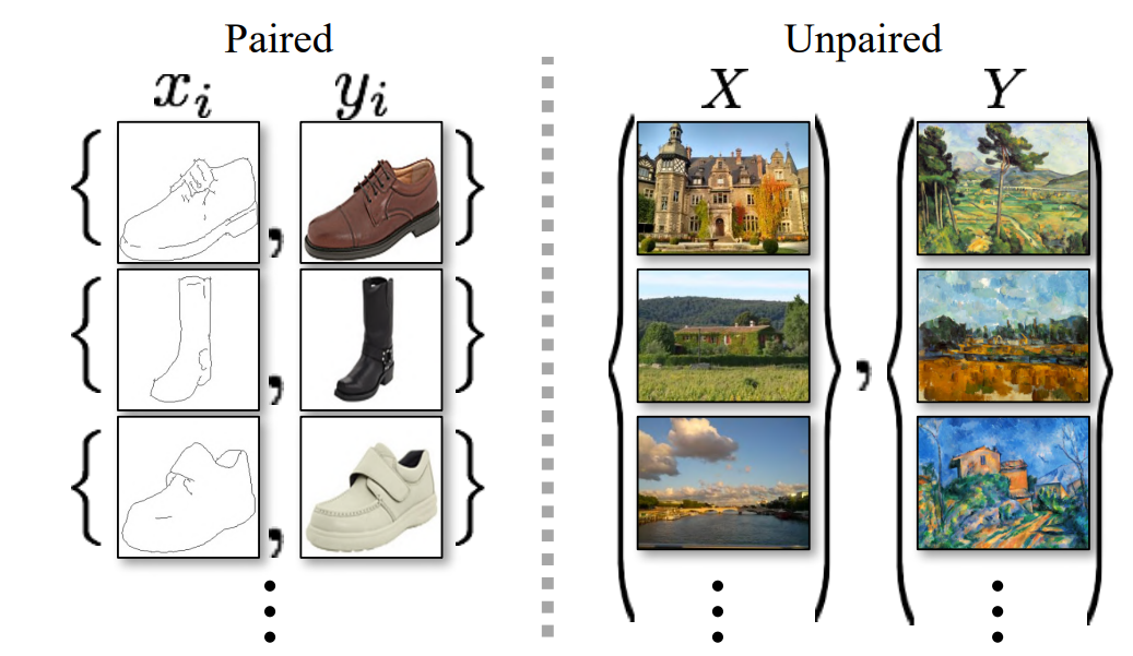
When we have specific conditions and proper pairing of data elements linking one image to its respective counterpart, it is easier to train such conditional GANs. Pix2Pix GANs are one such example where we work with paired images. Paired images are ones where the source image is linked to its corresponding target image. In paired image datasets, we have a clear mapping of both the source and target images, which are provided accordingly. However, such data is difficult to obtain in the real world.
Unpaired data, on the other hand, is relatively easier to obtain and can be found in abundance. In unpaired datasets, the source images and their corresponding target images are not directly provided. One of the primary approaches to solving projects or tasks related to unpaired datasets is to utilize Cycle-Consistent Adversarial Networks (Cycle GANs). Cycle GANs provide the user with an efficient method of achieving compelling results in most cases. In this research paper, most of the primary goals and accomplishments of this network are described in detail.
The Cycle GAN networks are capable of learning a mapping from image source $X$ to $Y$ from unpaired examples such that the generated images produced are of high quality. An additional cycle loss is also introduced in this research paper to confirm that the inverse mapping from the generated image reproduces the source image once again. Let us understand the working procedure and implementation details further in the upcoming section of this article.
Understanding Cycle GANs:
In this section, we will understand the detailed working explanation of Cycle GANs. In the introduction, we gently acknowledge that the application of Cycle GANs is primarily for unpaired image-to-image translations in opposition to other conditional GANs, such as pix2pix GANs. Let us try to understand the working procedure and the basic concepts of these networks, as well as gain a clear understanding of the generator and discriminator architecture.
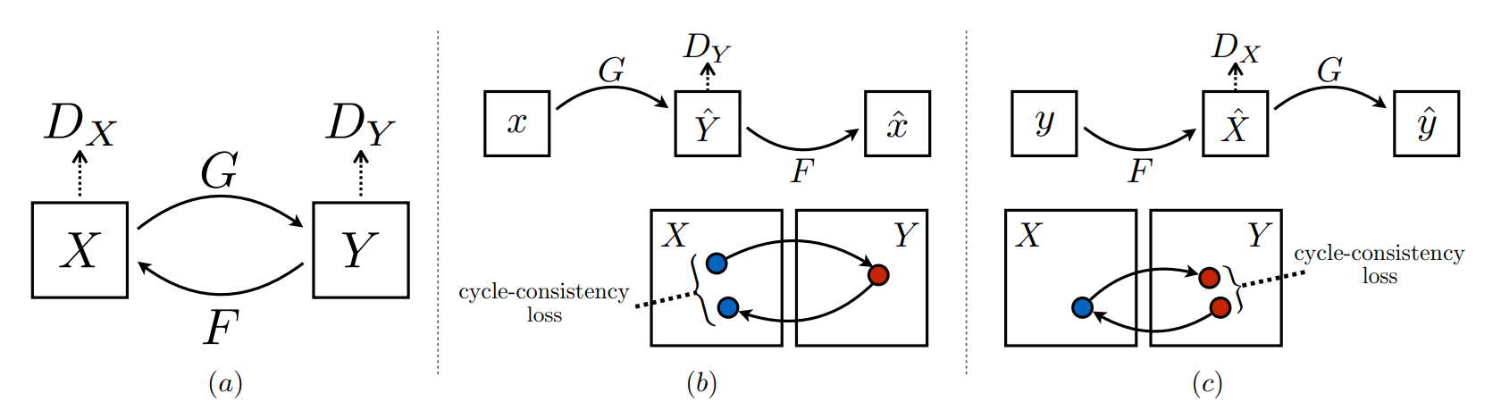
In the above image, let us consider the first sub-section with the generators $G$ and $F$ and the discriminators $Dx$ and $Dy$. The $X$ represents the input image, while the $Y$ represents the generated image. Unlike most GAN networks, which utilize a single generator and discriminator, the Cycle GAN network makes use of two generators and discriminators. The generator $G$ works on the input $X$ to generate an image $Y$. The discriminator $Dy$ distinguishes if the generated image is real or fake. Similarly, the generator $F$ generates an image $X$ considering an input $Y$. The discriminator $Dx$ distinguishes if this generated image is real or fake.
Apart from having a double generator and discriminator setup, we also have a cycle consistency loss to help the model to capture a greater intuitive understanding. If the model is trained on one source image to produce a generated image, then the cycle consistency loss ensures that when the generated image is translated back again into the original domain, we should be able to approximately retrieve the original source image once again.
In the above image, we can notice both the forward cycle-consistency loss and backward cycle-consistency loss in their respective sub-figures. Below is the final equation of all the loss functions combined for the Cycle GAN network. In this project, we also use an additional identity loss, which may not be required for most cases.
$$L(G, F, DX, DY ) = LGAN(G, DY , X, Y ) + LGAN(F, DX, Y, X) + λLcyc(G, F)$$
Now that we have understood the working procedure of these Cycle GAN networks, we can also briefly discuss the details behind the implementation of the generator and discriminator networks. The generator architecture comprises of three convolutional layers with varying filters, kernel sizes, and strides. After the three convolutional layers, we have the residual blocks. The network can either contain six or nine residual blocks.
At the end of the residual blocks, we make use of a couple of upsampling layers (or convolutional transpose layers) with a final convolutional layer resulting in the required image size for the generator. In the discriminator architecture, we have a simple 70 x 70 Patch GAN network, which contains four convolutional layers of increasing filter size. In these networks, instance normalization is preferred over batch normalization alongside Leaky ReLU activation functions. We will discuss more on the architectural details further when we construct these models from scratch.
Developing Unpaired Image To Image Translation using Cycle GANS:
In this section of the article, we will focus on developing the unpaired image-to-image translation project with the help of Cycle GANs. Now that we have a brief understanding of the basic working procedure of these Cycle-Consistent Adversarial Networks, we can build the overall architecture to process and compute the required task. We will utilize the TensorFlow and Keras deep learning frameworks for constructing these networks. If the viewers are not familiar with these libraries, I would recommend checking out a couple of my previous articles to gain more familiarity with these topics. You can check out the following article to learn more about TensorFlow and the Keras article here. Once done, we can start with the importing of the essential libraries.
Bring this project to life
Importing the essential libraries:
As discussed previously, one of the major changes from the previous pix2pix GAN architecture is the use of instance normalization layers over the batch normalization layers. Since there is no way to directly call the instance normalization layer through the existing Keras API, we will proceed to install an additional requirement. We will install the Keras-Contrib repository that will allow us to directly utilize these necessary layers without going through too much hassle.
pip install git+https://www.github.com/keras-team/keras-contrib.git
Once we have finished installing the pre-requisite requirement for the project, we can proceed to import all the essential libraries that we will utilize for constructing the Cycle GAN architecture and train the model accordingly to obtain the desired results. We will use the TensorFlow and Keras deep learning frameworks, as discussed previously, for building the network. We will use the functional API model type instead of the Sequential model to have overall higher control of the network design. We will also use a dataset that is available in the TensorFlow datasets library. Other necessary imports include matplotlib for visualization and the OS for handling tasks related to the local operating system. Below is the list of all the required imports.
import tensorflow as tf
from tensorflow.keras.optimizers import Adam
from tensorflow.keras.initializers import RandomNormal
from tensorflow.keras.models import Model
from tensorflow.keras.layers import Input, Conv2D, LeakyReLU, Conv2DTranspose
from tensorflow.keras.layers import Activation, Concatenate, BatchNormalization
from keras_contrib.layers.normalization.instancenormalization import InstanceNormalization
from tensorflow.keras.utils import plot_model
import tensorflow_datasets as tfds

import matplotlib.pyplot as plt
from IPython.display import clear_output
import time
import os

AUTOTUNE = tf.data.AUTOTUNE
Obtaining and preparing the dataset:
In this step, we will obtain the dataset for which we will perform the translation of images. We make use of the TensorFlow datasets library, through which we can retrieve all the relevant information. The dataset contains images of horses and zebras. For obtaining similar datasets for Cycle GAN projects, I would recommend checking out the following link. Below is the code snippet to load the datasets into their respective train and test variables.
dataset, metadata = tfds.load('cycle_gan/horse2zebra',
                              with_info=True, as_supervised=True)

train_horses, train_zebras = dataset['trainA'], dataset['trainB']
test_horses, test_zebras = dataset['testA'], dataset['testB']
Once we have retrieved the dataset, we can proceed to define some basic parameters that we will utilize for preparing the dataset.
BUFFER_SIZE = 1000
BATCH_SIZE = 1
IMG_WIDTH = 256
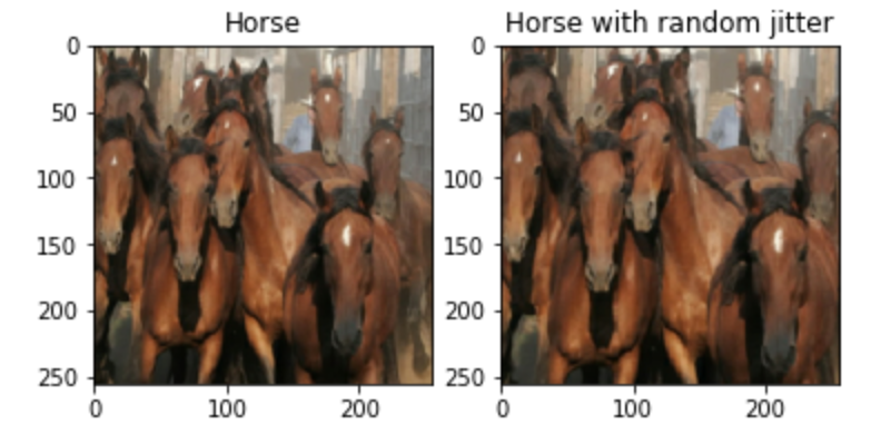
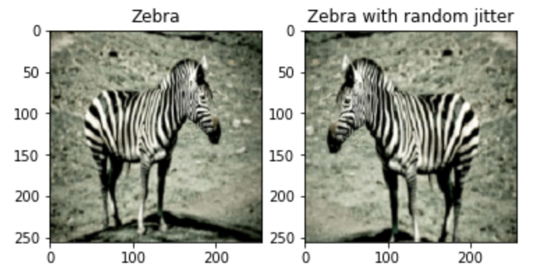
IMG_HEIGHT = 256In the next code block, we will define some basic functions for the dataset preparation. We will perform the normalization of the dataset to avoid extra memory usage and solve the task with relatively lesser resources. We will also apply jittering and mirroring to the existing data available, as suggested in the research paper, to avoid overfitting. Such augmentation techniques are usually quite useful. In this step, we are resizing the image to 286 x 286 and then cropping it back to the required 256 x 256 size, as well as flipping the images horizontally from left to right. Below is the code block for performing the following actions.
def random_crop(image):
    cropped_image = tf.image.random_crop(
      image, size=[IMG_HEIGHT, IMG_WIDTH, 3])

    return cropped_image

# normalizing the images to [-1, 1]
def normalize(image):
    image = tf.cast(image, tf.float32)
    image = (image / 127.5) - 1
    return image

def random_jitter(image):
    # resizing to 286 x 286 x 3
    image = tf.image.resize(image, [286, 286],
                          method=tf.image.ResizeMethod.NEAREST_NEIGHBOR)

    # randomly cropping to 256 x 256 x 3
    image = random_crop(image)

    # random mirroring
    image = tf.image.random_flip_left_right(image)

    return image

def preprocess_image_train(image, label):
    image = random_jitter(image)
    image = normalize(image)
    return image

def preprocess_image_test(image, label):
    image = normalize(image)
    return image
Finally, we will compute all these data elements into a final dataset. We will map the data with a random shuffle and pre-defined batch size through which all the components are accessible. We will define the dataset for all the training elements and testing ones for both the horse and zebra images, as shown in the below code snippet.
train_horses = train_horses.cache().map(
    preprocess_image_train, num_parallel_calls=AUTOTUNE).shuffle(
    BUFFER_SIZE).batch(BATCH_SIZE)

train_zebras = train_zebras.cache().map(
    preprocess_image_train, num_parallel_calls=AUTOTUNE).shuffle(
    BUFFER_SIZE).batch(BATCH_SIZE)

test_horses = test_horses.map(
    preprocess_image_test, num_parallel_calls=AUTOTUNE).cache().shuffle(
    BUFFER_SIZE).batch(BATCH_SIZE)

test_zebras = test_zebras.map(
    preprocess_image_test, num_parallel_calls=AUTOTUNE).cache().shuffle(
    BUFFER_SIZE).batch(BATCH_SIZE)

sample_horse = next(iter(train_horses))
sample_zebra = next(iter(train_zebras))
Below are some sample images with the datasets containing the original image and its corresponding image with some random jitter.
Once we have completed all the required steps for obtaining and preparing the dataset, we can proceed to create the discriminator and generator networks to build the overall Cycle GAN architecture.
Define the discriminator architecture:
For the discriminator architecture, we have four convolutional blocks defined as follows - $C64-C128-C256-C512$. The Leaky ReLU activation function with an alpha (slope) value of 0.2 is used. Except for the first convolutional block, all other blocks make use of an instance normalization right after the convolutional layers. The strides and kernel sizes are as shown in the code snippet below. We will finally compile the model with a mean square error loss function and an Adam optimizer to complete the Patch GAN discriminator type network.
# define the discriminator model
def define_discriminator(image_shape):
    # weight initialization
    init = RandomNormal(stddev=0.02)
    # source image input
    in_image = Input(shape=image_shape)
    # C64
    d = Conv2D(64, (4,4), strides=(2,2), padding='same', kernel_initializer=init)(in_image)
    d = LeakyReLU(alpha=0.2)(d)
    # C128
    d = Conv2D(128, (4,4), strides=(2,2), padding='same', kernel_initializer=init)(d)
    d = InstanceNormalization(axis=-1)(d)
    d = LeakyReLU(alpha=0.2)(d)
    # C256
    d = Conv2D(256, (4,4), strides=(2,2), padding='same', kernel_initializer=init)(d)
    d = InstanceNormalization(axis=-1)(d)
    d = LeakyReLU(alpha=0.2)(d)
    # C512
    d = Conv2D(512, (4,4), strides=(2,2), padding='same', kernel_initializer=init)(d)
    d = InstanceNormalization(axis=-1)(d)
    d = LeakyReLU(alpha=0.2)(d)
    # second last output layer
    d = Conv2D(512, (4,4), padding='same', kernel_initializer=init)(d)
    d = InstanceNormalization(axis=-1)(d)
    d = LeakyReLU(alpha=0.2)(d)
    # patch output
    patch_out = Conv2D(1, (4,4), padding='same', kernel_initializer=init)(d)
    # define model
    model = Model(in_image, patch_out)
    # compile model
    model.compile(loss='mse', optimizer=Adam(learning_rate=0.0002, beta_1=0.5), loss_weights=[0.5])
    return model

# define image shape
image_shape = (256,256,3)

# create the model
model = define_discriminator(image_shape)

# summarize the model
model.summary()
Define the Generator architecture:
The generator architecture consists of one convolutional block with 64 filters and a 7 x 7 kernel size with a stride of 2, followed by two convolutional layers of 3 x 3 kernel size with a stride of 1, respectively, with 128 and 256 filters. We will then define the residual block, which is nothing but a bunch of convolutional layers. This residual block is followed by a couple of upsampling layers defined by the Convolutional 2D Transpose layers. The final convolutional layer contains a 7 x 7 kernel size with a stride of 1 and 3 filters.
They generator architecture for 9 residual blocks is defined as follows: $c7s1-64, d128, d256, R256, R256, R256, R256, R256, R256, R256, R256, R256, u128, u64, c7s1-3$
# generator a resnet block
def resnet_block(n_filters, input_layer):
    # weight initialization
    init = RandomNormal(stddev=0.02)
    # first layer convolutional layer
    g = Conv2D(n_filters, (3,3), padding='same', kernel_initializer=init)(input_layer)
    g = InstanceNormalization(axis=-1)(g)
    g = Activation('relu')(g)
    # second convolutional layer
    g = Conv2D(n_filters, (3,3), padding='same', kernel_initializer=init)(g)
    g = InstanceNormalization(axis=-1)(g)
    # concatenate merge channel-wise with input layer
    g = Concatenate()([g, input_layer])
    return g

# define the standalone generator model
def define_generator(image_shape=(256, 256, 3), n_resnet=9):
    # weight initialization
    init = RandomNormal(stddev=0.02)
    # image input
    in_image = Input(shape=image_shape)
    # c7s1-64
    g = Conv2D(64, (7,7), padding='same', kernel_initializer=init)(in_image)
    g = InstanceNormalization(axis=-1)(g)
    g = Activation('relu')(g)
    # d128
    g = Conv2D(128, (3,3), strides=(2,2), padding='same', kernel_initializer=init)(g)
    g = InstanceNormalization(axis=-1)(g)
    g = Activation('relu')(g)
    # d256
    g = Conv2D(256, (3,3), strides=(2,2), padding='same', kernel_initializer=init)(g)
    g = InstanceNormalization(axis=-1)(g)
    g = Activation('relu')(g)
    # R256
    for _ in range(n_resnet):
        g = resnet_block(256, g)
    # u128
    g = Conv2DTranspose(128, (3,3), strides=(2,2), padding='same', kernel_initializer=init)(g)
    g = InstanceNormalization(axis=-1)(g)
    g = Activation('relu')(g)
    # u64
    g = Conv2DTranspose(64, (3,3), strides=(2,2), padding='same', kernel_initializer=init)(g)
    g = InstanceNormalization(axis=-1)(g)
    g = Activation('relu')(g)
    # c7s1-3
    g = Conv2D(3, (7,7), padding='same', kernel_initializer=init)(g)
    g = InstanceNormalization(axis=-1)(g)
    out_image = Activation('tanh')(g)
    # define model
    model = Model(in_image, out_image)
    return model

# create the model
model = define_generator()
# summarize the model
model.summary()
Defining loss function and checkpoints:
In the next code snippet, we will explore the different types of loss functions that we will utilize for the Cycle GAN architecture. We will define generator loss, discriminator loss, cycle consistency loss, and identity loss. The reason for the cycle consistency loss, as discussed previously, is to maintain an approximate relationship between the source image and the reproduced image. Finally, we will define the Adam optimizers for both the generator and discriminator networks, as shown in the below code block.
LAMBDA = 10

loss_obj = tf.keras.losses.BinaryCrossentropy(from_logits=True)

def discriminator_loss(real, generated):
    real_loss = loss_obj(tf.ones_like(real), real)

    generated_loss = loss_obj(tf.zeros_like(generated), generated)

    total_disc_loss = real_loss + generated_loss

    return total_disc_loss * 0.5

def generator_loss(generated):
    return loss_obj(tf.ones_like(generated), generated)

def calc_cycle_loss(real_image, cycled_image):
    loss1 = tf.reduce_mean(tf.abs(real_image - cycled_image))

    return LAMBDA * loss1

def identity_loss(real_image, same_image):
    loss = tf.reduce_mean(tf.abs(real_image - same_image))
    return LAMBDA * 0.5 * loss

generator_g_optimizer = tf.keras.optimizers.Adam(2e-4, beta_1=0.5)
generator_f_optimizer = tf.keras.optimizers.Adam(2e-4, beta_1=0.5)

discriminator_x_optimizer = tf.keras.optimizers.Adam(2e-4, beta_1=0.5)
discriminator_y_optimizer = tf.keras.optimizers.Adam(2e-4, beta_1=0.5)
Once we have finished defining the loss functions and optimizers, we will also define a checkpoint system where we will store the desired checkpoint with the most recent results being saved. We can do this to allow us to reload and retrain the weights if needed.
checkpoint_path = "./checkpoints/train"

ckpt = tf.train.Checkpoint(generator_g=generator_g,
                           generator_f=generator_f,
                           discriminator_x=discriminator_x,
                           discriminator_y=discriminator_y,
                           generator_g_optimizer=generator_g_optimizer,
                           generator_f_optimizer=generator_f_optimizer,
                           discriminator_x_optimizer=discriminator_x_optimizer,
                           discriminator_y_optimizer=discriminator_y_optimizer)

ckpt_manager = tf.train.CheckpointManager(ckpt, checkpoint_path, max_to_keep=5)

# if a checkpoint exists, restore the latest checkpoint.
if ckpt_manager.latest_checkpoint:
    ckpt.restore(ckpt_manager.latest_checkpoint)
    print ('Latest checkpoint restored!!')
Define the final training function:
In the final step, we will define the training function to train our model and generate the desired images as required. Firstly, let us set the number of epochs that we plan to train the model for and create a function for creating the respective plots for visualizing the input and predicted image. Note that for this training, I used a keyboard interrupt after twenty epochs, but the viewers can train for longer periods to achieve better results.
EPOCHS = 50

def generate_images(model, test_input):
    prediction = model(test_input)

    plt.figure(figsize=(12, 12))

    display_list = [test_input[0], prediction[0]]
    title = ['Input Image', 'Predicted Image']

    for i in range(2):
        plt.subplot(1, 2, i+1)
        plt.title(title[i])
        # getting the pixel values between [0, 1] to plot it.
        plt.imshow(display_list[i] * 0.5 + 0.5)
        plt.axis('off')
    plt.show()
In the training step function, we will call the tf.function and Gradient tape for faster training computation of the backpropagation weights. The training method is similar to the previous GAN architectures that we have previously built with the exception that we will train two generators and discriminators in this method as well as evaluate the cycle consistency loss as required. Below is the code block for the complete training procedure of the Cycle GAN architecture.
@tf.function
def train_step(real_x, real_y):
  # persistent is set to True because the tape is used more than
  # once to calculate the gradients.
    with tf.GradientTape(persistent=True) as tape:
        # Generator G translates X -> Y
        # Generator F translates Y -> X.

        fake_y = generator_g(real_x, training=True)
        cycled_x = generator_f(fake_y, training=True)

        fake_x = generator_f(real_y, training=True)
        cycled_y = generator_g(fake_x, training=True)

        # same_x and same_y are used for identity loss.
        same_x = generator_f(real_x, training=True)
        same_y = generator_g(real_y, training=True)

        disc_real_x = discriminator_x(real_x, training=True)
        disc_real_y = discriminator_y(real_y, training=True)

        disc_fake_x = discriminator_x(fake_x, training=True)
        disc_fake_y = discriminator_y(fake_y, training=True)

        # calculate the loss
        gen_g_loss = generator_loss(disc_fake_y)
        gen_f_loss = generator_loss(disc_fake_x)

        total_cycle_loss = calc_cycle_loss(real_x, cycled_x) + calc_cycle_loss(real_y, cycled_y)

        # Total generator loss = adversarial loss + cycle loss
        total_gen_g_loss = gen_g_loss + total_cycle_loss + identity_loss(real_y, same_y)
        total_gen_f_loss = gen_f_loss + total_cycle_loss + identity_loss(real_x, same_x)

        disc_x_loss = discriminator_loss(disc_real_x, disc_fake_x)
        disc_y_loss = discriminator_loss(disc_real_y, disc_fake_y)

    # Calculate the gradients for generator and discriminator
    generator_g_gradients = tape.gradient(total_gen_g_loss,
                                        generator_g.trainable_variables)
    generator_f_gradients = tape.gradient(total_gen_f_loss,
                                        generator_f.trainable_variables)

    discriminator_x_gradients = tape.gradient(disc_x_loss,
                                            discriminator_x.trainable_variables)
    discriminator_y_gradients = tape.gradient(disc_y_loss,
                                            discriminator_y.trainable_variables)

    # Apply the gradients to the optimizer
    generator_g_optimizer.apply_gradients(zip(generator_g_gradients,
                                            generator_g.trainable_variables))

    generator_f_optimizer.apply_gradients(zip(generator_f_gradients,
                                            generator_f.trainable_variables))

    discriminator_x_optimizer.apply_gradients(zip(discriminator_x_gradients,
                                                discriminator_x.trainable_variables))

    discriminator_y_optimizer.apply_gradients(zip(discriminator_y_gradients,
                                                discriminator_y.trainable_variables))
Finally, we can start the training process for the defined number of epochs. We will loop through our training data and train the model accordingly. At the end of each epoch, we can generate the resulting image to notice the progression made by the model. We can also save the checkpoints, as shown in the code snippet below.
for epoch in range(EPOCHS):
    start = time.time()

    n = 0
    for image_x, image_y in tf.data.Dataset.zip((train_horses, train_zebras)):
        train_step(image_x, image_y)
        if n % 10 == 0:
            print ('.', end='')
        n += 1

    clear_output(wait=True)
    # Using a consistent image (sample_horse) so that the progress of the model
    # is clearly visible.
    generate_images(generator_g, sample_horse)

    if (epoch + 1) % 5 == 0:
        ckpt_save_path = ckpt_manager.save()
        print ('Saving checkpoint for epoch {} at {}'.format(epoch+1,
                                                         ckpt_save_path))

    print ('Time taken for epoch {} is {} sec\n'.format(epoch + 1,
                                                      time.time()-start))
Saving checkpoint for epoch 20 at ./checkpoints/train/ckpt-4
Below are some of the results that I was able to obtain after twenty epochs of training. Training for a higher number of epochs and varying a few parameters could yield even better results.
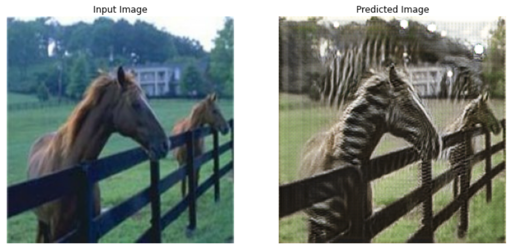
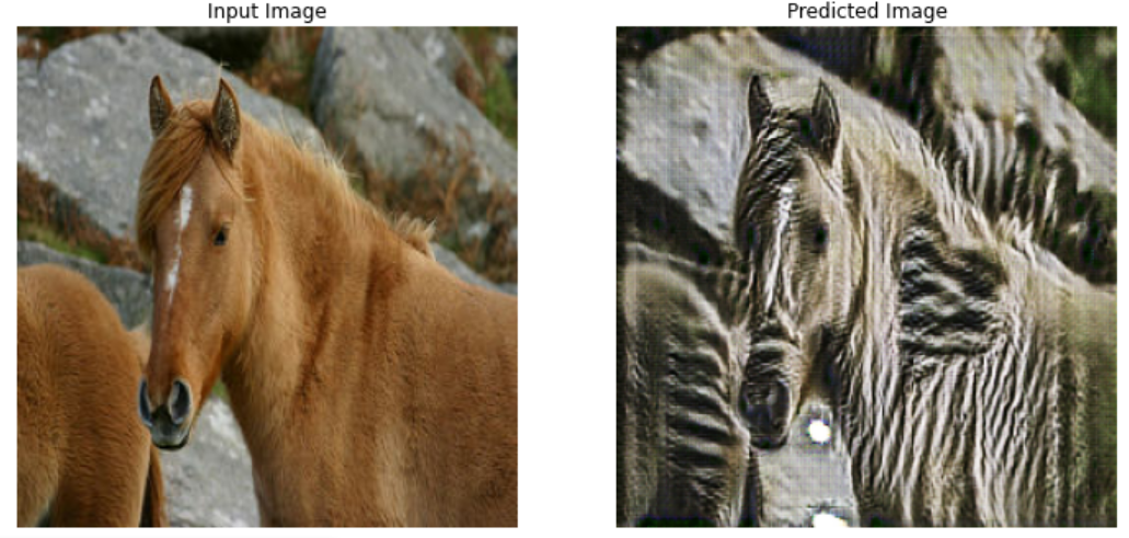
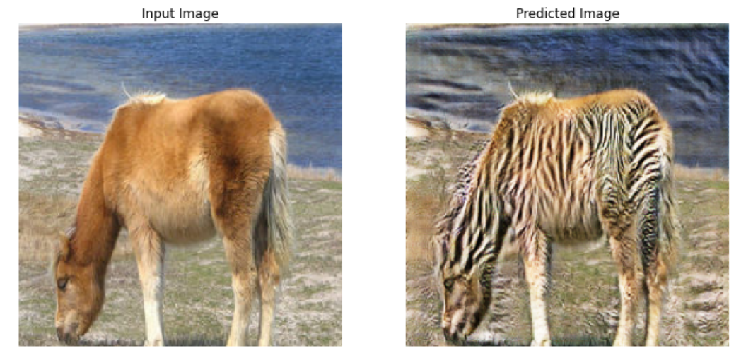
With the help of Cycle GANs, we can notice the overall results obtained with the trained architecture are quite compelling. We are able to produce the desired results for the unpaired image translation task to an obviously interpretable degree. While there are a few limitations of this network, including the loss of background color and texture details, we are still able to retrieve approximately most of the necessary information for the particular task. I would recommend trying out numerous parameters, variations, and minor architectural changes to achieve more optimal results.
The major portions of this code are considered from the official TensorFlow website, which can be viewed from this link. However, they utilize a variation of the pix-2-pix model for training the Cycle GAN network for simplicity making use of a U-Net-like generator network and the corresponding discriminator network. In this article, we solely focused on reconstructing the research paper from scratch and used the ResNet architecture for the generator and the slightly modified Patch GAN architecture for the discriminator. I would recommend checking out the following reference link for a more detailed guide on only the Cycle GAN generator and discriminator implementation.
Conclusion:

In the natural world, it is difficult to obtain a large dataset of paired examples for complex problems. Creating such paired datasets linking source image to their respective target images are often expensive and time-consuming. However, a large number of unpaired examples of image-to-image translations are available over the internet. The horse and zebra dataset discussed in this article is one such example where the desired output is not clearly well defined. Most modern GANs can solve tasks and projects related to paired examples on image-to-image translations. But the Cycle GAN conditional GAN has the ability to achieve desirable outputs on unpaired datasets.
In this article, we explored another variation of conditional GANs in Cycle-Consistent Adversarial Networks (Cycle GANs). We understood how powerful these GANs are and their ability to learn image-to-image translations even in the absence of paired examples. We had a brief introduction of some of the basic concepts of these Cycle GANs, along with a detailed breakdown of some of the core concepts of their network architecture. Finally, we concluded our conceptual understanding with the development of the "Unpaired Image-To-Image Translation using Cycle GANS" project from scratch.
In future articles, we will cover more types of GANs, such as ProGAN, StyleGAN, and so much more. We will also experiment with some audio tasks with deep learning and learn about constructing neural networks from scratch. Until then, keep learning and exploring!