Since 2014, Generative Adversarial Networks (GANs) have been taking over the field of deep learning and neural networks due to the immense potential these architectures possess. While the initial GANs were able to produce decent results, they were often found to fail when trying to perform more difficult computations. Hence, several variations of these GANs have been proposed to ensure that we are able to achieve the best results possible. In our previous articles, we have covered such versions of GANs to solve different types of projects, and in this article, we will also do the same.
In this article, we will cover one of the types of generative adversarial networks (GANs) in Wasserstein GAN (WGANs). We will understand the working of these WGAN generators and discriminator structures as well as dwell on the details for their implementation. We will look into its implementation with the gradient penalty approach, and, finally, construct a project with the following architecture from scratch. The entire project can be implemented on the Gradient platform available on Paperspace. For viewers who want to train the project, I would recommend the viewers to check out the website and implement the project alongside.
Introduction:
Generative Adversarial Networks (GANs) are a tremendous accomplishment in the world of artificial intelligence and deep learning. Since their original introduction, they have been consistently used in the development of spectacular projects. While these GANs, with their competing generator and discriminator models, are able to achieve massive success, there were several cases of failure of these networks.
Two of the most common reasons were due to either a convergence failure or a mode collapse. In convergence failure, the model failed to produce optimal or good quality results. In the case of a mode collapse, the model failed to produce unique images repeating a similar pattern or quality. Hence, to solve some of these issues or to combat numerous types of problems, there were gradually many variations and versions developed for GANs.
While we have discussed the concept of DCGANs in some of our previous articles, in this blog, we will focus on the WGAN networks for combating such issues. WGAN offers higher stability to the training model in comparison to simple GAN architectures. The loss function utilized in WGAN also gives us a termination criterion for evaluating the model. While it may sometimes take slightly longer to train, it is one of the better options to achieve more efficient results. Let us understand the concept of these WGANs in a bit more detail in the next section.
Understanding WGANs:
The idea for the working of Generative Adversarial Networks (GANs) is to utilize two primary probability distributions. One of the main entity is the probability distribution of the generator (Pg), which refers to the distribution from the output of the generator model. The other essential entity is the probability distribution from the real images (Pr). The objective of the Generative Adversarial Networks is to ensure that both these probability distributions are close to each other so that the output generated is highly realistic and high-quality.
For calculating the distance of these probability distributions, mathematical statistics in machine learning proposes three primary methods, namely Kullback–Leibler divergence, Jensen–Shannon divergence, and Wasserstein distance. The Jensen–Shannon divergence (also a typical GAN loss) is initially the more utilized mechanism in simple GAN networks.
However, this method has issues while working with gradients that can lead to unstable training. Hence, we make use of the Wasserstein distance to fix such recurring issues. The representation for the mathematical formula is as shown below. Refer to the following research paper for further reading and information.
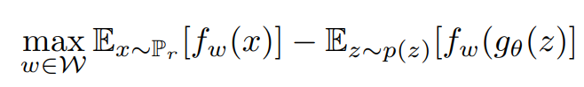
In the above equation, the max value represents the constraint on the discriminator. In the WGAN architecture, the discriminator is referred to as the critic. One of the reasons for this convention is that there is no sigmoid activation function to limit the values to 0 or 1, which means real or fake. Instead, the WGAN discriminator networks return a value in a range, which allows it to act less strictly as a critic.
The first part of the equation represents the real data, while the second half represents the generator data. The discriminator (or the critic) in the above equation aims to maximize the distance between the real data and the generated data because it wants to be able to successfully distinguish the data accordingly. The generator network aims to minimize the distance between the real data and generated data because it wants the generated data to be as real as possible.
Learning the details for the implementation of WGANs:
For the original implementation of the WGAN network, I would recommend checking out the following research paper. It describes the implementation of the architectural build in detail. The critic adds a meaningful metric for the desired computation for problems related to GAN and also improves the training stability.
However, one of the main disadvantages of the initial research paper, which uses a method of weight clipping, was found to be that this method did not always work as optimally as expected. When the weight clipping was sufficiently large, it led to longer training times as the critic took a lot of time to adjust to the expected weights. When the weight clipping was small, it led to vanishing gradients, especially in cases of a large number of layers, no batch normalization, or problems related to RNNs.
Hence, there was a need for a slight improvement in the training mechanism of WGAN. One of the best methods introduced to combat these issues was in the following research paper which tackled this problem with the use of the gradient penalty method. This research paper help in improving the training of the WGAN. Let us look at an image of the algorithm that is proposed for achieving the required task.
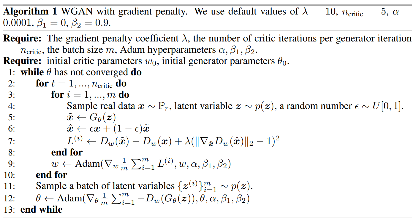
The WGAN uses a gradient penalty approach to effectively solve the previous issues of this network. The WGAN-GP method proposes an alternative to weight clipping to ensure smooth training. Instead of clipping the weights, the authors proposed a "gradient penalty" by adding a loss term that keeps the L2 norm of the discriminator gradients close to 1 (Source). The algorithm above defines some of the basic parameters that we must consider while utilizing this approach.
The lambda defines the gradient penalty coefficient, while the n-critic refers to the number of critic iteration per generator iteration. The alpha and beta values refer to the constraints of the Adam optimizer. The approach proposes that we make use of an interpolation image alongside the generated image before adding the loss function with gradient penalty as it helps to satisfy the Lipschitz constraint. The algorithm is run until we are able to achieve a satisfactory convergence on the required data. Let us now look at the practical implementation of this WGAN with the gradient penalty method for constructing the MNIST project.
Construct a project with WGANs:
In this section of the article, we will develop the WGAN networks from our understanding of the method of functioning and details of implementation. We will ensure that we use a gradient penalty methodology while training the WGAN network. For the construction of this project, we will utilize the following reference link from the official Keras website, from which a majority of the code has been considered.
If you are working within Gradient, I suggest you create a Notebook using the TensorFlow runtime. This will set up your environment in a docker container with TensorFlow and Keras installed.
Bring this project to life
Importing the essential libraries:
We will make use of the TensorFlow and Keras deep learning frameworks for constructing the WGAN architecture. If you are not too familiar with these libraries, I will recommend referring to my previous articles that cover these two topics extensively. The viewers can check out the TensorFlow article from this link and the Keras blog from the following link. These two libraries should be sufficient for the construction of most of the tasks in this project. We will also import numpy for some array computations and matplotlib for some visualizations if required.
import tensorflow as tf
from tensorflow import keras
from tensorflow.keras import layers
import matplotlib.pyplot as plt
import numpy as np
Defining Parameters and Loading Data:
In this section, we will define some of the basic parameters, define a few blocks of neural networks to reuse throughout the project, namely the conv block and the upsample block and load the MNIST data accordingly. Let us first define some of the parameters, such as the image size of the MNIST data, which is 28 x 28 x 1 because each image has a height and width of 28 and has one channel, which means it is a grayscale image. Let us also define a base batch size and a noise dimension which the generator can utilize for the generation of the desired number of 'digit' images.
IMG_SHAPE = (28, 28, 1)
BATCH_SIZE = 512
noise_dim = 128
In the next step, we will load the MNIST data, which is directly accessible from the TensorFlow and Keras datasets free example datasets. We will divide the 60000 existing images equivalently into their respective train images, train labels, test images, and test labels. Finally, we will normalize these images so that the training model can easily compute the values in the specific range. Below is the code block for performing the following actions.
MNIST_DATA = keras.datasets.mnist

(train_images, train_labels), (test_images, test_labels) = MNIST_DATA.load_data()

print(f"Number of examples: {len(train_images)}")
print(f"Shape of the images in the dataset: {train_images.shape[1:]}")

train_images = train_images.reshape(train_images.shape[0], *IMG_SHAPE).astype("float32")
train_images = (train_images - 127.5) / 127.5
In the next code snippet, we will define the convolutional block, which we will mostly utilize for the construction of the discriminator architecture for it to act as a critic for the generated images. The convolutional block function will take in some of the basic parameters for the convolution 2D layer as well as some other parameters, namely batch normalization, and dropout. As described in the research paper, some of the layers of the discriminator critic model make use of a batch normalization or dropout layer. Hence, we can choose to add either of the two layers to be followed after a convolutional layer if required. The code snippet below represents the function for the convolutional block.
def conv_block(x, filters, activation, kernel_size=(3, 3), strides=(1, 1), padding="same",
               use_bias=True, use_bn=False, use_dropout=False, drop_value=0.5):

    x = layers.Conv2D(filters, kernel_size, strides=strides,
                      padding=padding, use_bias=use_bias)(x)

    if use_bn:
        x = layers.BatchNormalization()(x)
    x = activation(x)
    if use_dropout:
        x = layers.Dropout(drop_value)(x)

    return x
Similarly, we will also construct another function for the upsample block, which we will mostly utilize throughout the computation of the generator architecture of the WGAN structure. We will define some of the basic parameters and an option if we want to include the batch normalization layer or the dropout layer. Note that each upsample block is followed by a conventional convolutional layer as well. The batch normalization or dropout layer may be added after these two layers if required. Check out the below code for creating the upsample block.
def upsample_block(x, filters, activation, kernel_size=(3, 3), strides=(1, 1), up_size=(2, 2), padding="same",
                   use_bn=False, use_bias=True, use_dropout=False, drop_value=0.3):

    x = layers.UpSampling2D(up_size)(x)
    x = layers.Conv2D(filters, kernel_size, strides=strides,
                      padding=padding, use_bias=use_bias)(x)

    if use_bn:
        x = layers.BatchNormalization()(x)

    if activation:
        x = activation(x)
    if use_dropout:
        x = layers.Dropout(drop_value)(x)

    return x
In the next couple of sections, we will utilize both the convolutional block and the upsample blocks to construct the generator and discriminator architecture. Let us proceed to look at how to build the generator model and the discriminator model accordingly to create an overall highly effective WGAN architecture to solve the MNIST project.
Constructing The Generator Architecture:
With the help of the previously defined functions of the upsample blocks, we can proceed to construct our generator model for working with this project. We will now define some basic requirements, such as the noise with the latent dimension that we previously assigned. We will follow this noise up with a fully connected layer, a batch normalization layer, and a Leaky ReLU. Before we pass the output to the next upsample blocks, we need to reshape the function accordingly.
We will then pass the reshaped noise output into a series of upsampling blocks. Once we pass the output through three upsample blocks, we achieve a final shape of 32 x 32 in the height and width dimension. But we know that the shape of the MNIST dataset is in the form of 28x28. To achieve this data, we will use the Cropping 2D layer for achieving the required shape. Finally, we will finish the construction of the generator architecture by calling the model function.
def get_generator_model():
    noise = layers.Input(shape=(noise_dim,))
    x = layers.Dense(4 * 4 * 256, use_bias=False)(noise)
    x = layers.BatchNormalization()(x)
    x = layers.LeakyReLU(0.2)(x)

    x = layers.Reshape((4, 4, 256))(x)

    x = upsample_block(x, 128, layers.LeakyReLU(0.2), strides=(1, 1), use_bias=False,
                       use_bn=True, padding="same", use_dropout=False)

    x = upsample_block(x, 64, layers.LeakyReLU(0.2), strides=(1, 1), use_bias=False,
                       use_bn=True, padding="same", use_dropout=False)

    x = upsample_block(x, 1, layers.Activation("tanh"), strides=(1, 1),
                       use_bias=False, use_bn=True)

    x = layers.Cropping2D((2, 2))(x)

    g_model = keras.models.Model(noise, x, name="generator")
    return g_model


g_model = get_generator_model()
g_model.summary()
Bring this project to life
Constructing The Discriminator Architecture:
Now that we have completed the construction of the generator architecture, we can proceed to create the discriminator network (more commonly known as the critic in WGANs). The first step we will perform in the discriminator model for performing the project of MNIST data generation is to adjust the shape accordingly. Since the dimensions of 28 x 28 lead to an odd dimension after a couple of strides, it is best to convert the image size into the dimension of 32 x 32 because it provides an even dimension after performing the striding operation.
Once we add the zero-padding layer, we can continue to develop the critic architecture as desired. We will then proceed to add a series of convolutional blocks as described in our previous function. Note the layers that may or may not use a batch normalization or dropout layer. After four convolutional blocks, we will pass the output through a flatten layer, a dropout layer, and finally, a dense layer. Note that the dense layer does not utilize a sigmoid activation function, unlike other discriminators in simple GAN networks. Finally, call the model to create the critic network.
def get_discriminator_model():

    img_input = layers.Input(shape=IMG_SHAPE)
    x = layers.ZeroPadding2D((2, 2))(img_input)

    x = conv_block(x, 64, kernel_size=(5, 5), strides=(2, 2), use_bn=False, use_bias=True,
                   activation=layers.LeakyReLU(0.2), use_dropout=False, drop_value=0.3)

    x = conv_block(x, 128, kernel_size=(5, 5), strides=(2, 2), use_bn=False, use_bias=True,
                   activation=layers.LeakyReLU(0.2), use_dropout=True, drop_value=0.3)

    x = conv_block(x, 256, kernel_size=(5, 5), strides=(2, 2), use_bn=False, use_bias=True,
                   activation=layers.LeakyReLU(0.2), use_dropout=True, drop_value=0.3)

    x = conv_block(x, 512, kernel_size=(5, 5), strides=(2, 2), use_bn=False, use_bias=True,
                   activation=layers.LeakyReLU(0.2), use_dropout=False, drop_value=0.3)


    x = layers.Flatten()(x)
    x = layers.Dropout(0.2)(x)
    x = layers.Dense(1)(x)

    d_model = keras.models.Model(img_input, x, name="discriminator")
    return d_model


d_model = get_discriminator_model()
d_model.summary()
Creating the overall WGAN model:
Over next step is to define the overall Wasserstein GAN network. We will divide this WGAN building structure into the form of three blocks. In the first code block, we will define all the parameters that we will utilize throughout the class in various functions. Check the code snippet below to gain an understanding of the different parameters that we will utilize. Note that all the functions are to be inside the WGAN class.
class WGAN(keras.Model):
    def __init__(self, discriminator, generator, latent_dim,
                 discriminator_extra_steps=3, gp_weight=10.0):
        super(WGAN, self).__init__()

        self.discriminator = discriminator
        self.generator = generator
        self.latent_dim = latent_dim
        self.d_steps = discriminator_extra_steps
        self.gp_weight = gp_weight

    def compile(self, d_optimizer, g_optimizer, d_loss_fn, g_loss_fn):
        super(WGAN, self).compile()
        self.d_optimizer = d_optimizer
        self.g_optimizer = g_optimizer
        self.d_loss_fn = d_loss_fn
        self.g_loss_fn = g_loss_fn
In the next function, we will create the gradient penalty method that we have discussed in the previous section. Note that the gradient penalty loss is calculated on an interpolated image and added to the discriminator loss as discussed in the algorithm of the previous section. This method allows us to achieve faster convergence and higher stability while training. It also enables us to achieve a better assignment of weights. Check the below code for the implementation of the gradient penalty.
    def gradient_penalty(self, batch_size, real_images, fake_images):
        # Get the interpolated image
        alpha = tf.random.normal([batch_size, 1, 1, 1], 0.0, 1.0)
        diff = fake_images - real_images
        interpolated = real_images + alpha * diff

        with tf.GradientTape() as gp_tape:
            gp_tape.watch(interpolated)
            pred = self.discriminator(interpolated, training=True)

        grads = gp_tape.gradient(pred, [interpolated])[0]
        norm = tf.sqrt(tf.reduce_sum(tf.square(grads), axis=[1, 2, 3]))
        gp = tf.reduce_mean((norm - 1.0) ** 2)
        return gp
In the next and final function, we will define the training step for the WGAN architecture similar to the algorithm specified in the previous section. We will first train the generator and achieve the loss for the generator. We will then train the critic model and obtain the loss for the discriminator. Once we know the losses for both the generator and the critic, we will interpret the gradient penalty. Once the gradient penalty is calculated, we will multiply it with a constant weight factor and this gradient penalty to the critic. Finally, we will return the generator and critic losses accordingly. The below code snippet defines how the following actions can be performed.
    def train_step(self, real_images):
        if isinstance(real_images, tuple):
            real_images = real_images[0]

        batch_size = tf.shape(real_images)[0]

        for i in range(self.d_steps):
            # Get the latent vector
            random_latent_vectors = tf.random.normal(
                shape=(batch_size, self.latent_dim)
            )
            with tf.GradientTape() as tape:
                # Generate fake images from the latent vector
                fake_images = self.generator(random_latent_vectors, training=True)
                # Get the logits for the fake images
                fake_logits = self.discriminator(fake_images, training=True)
                # Get the logits for the real images
                real_logits = self.discriminator(real_images, training=True)

                # Calculate the discriminator loss using the fake and real image logits
                d_cost = self.d_loss_fn(real_img=real_logits, fake_img=fake_logits)
                # Calculate the gradient penalty
                gp = self.gradient_penalty(batch_size, real_images, fake_images)
                # Add the gradient penalty to the original discriminator loss
                d_loss = d_cost + gp * self.gp_weight

            # Get the gradients w.r.t the discriminator loss
            d_gradient = tape.gradient(d_loss, self.discriminator.trainable_variables)
            # Update the weights of the discriminator using the discriminator optimizer
            self.d_optimizer.apply_gradients(zip(d_gradient, self.discriminator.trainable_variables))

        # Train the generator
        random_latent_vectors = tf.random.normal(shape=(batch_size, self.latent_dim))
        with tf.GradientTape() as tape:
            # Generate fake images using the generator
            generated_images = self.generator(random_latent_vectors, training=True)
            # Get the discriminator logits for fake images
            gen_img_logits = self.discriminator(generated_images, training=True)
            # Calculate the generator loss
            g_loss = self.g_loss_fn(gen_img_logits)

        # Get the gradients w.r.t the generator loss
        gen_gradient = tape.gradient(g_loss, self.generator.trainable_variables)
        # Update the weights of the generator using the generator optimizer
        self.g_optimizer.apply_gradients(zip(gen_gradient, self.generator.trainable_variables))
        return {"d_loss": d_loss, "g_loss": g_loss}
Training the model:
The final step of developing the WGAN architecture and solving our project is to train it effectively and achieve the desired result. We will divide this section into a few functions. In the first function, we will proceed to create the custom callback for the WGAN model. Using this custom callback that we create, we can save the generated images periodically. The code snippet below shows how you can create your own custom callbacks to perform a specific operation.
class GANMonitor(keras.callbacks.Callback):
    def __init__(self, num_img=6, latent_dim=128):
        self.num_img = num_img
        self.latent_dim = latent_dim

    def on_epoch_end(self, epoch, logs=None):
        random_latent_vectors = tf.random.normal(shape=(self.num_img, self.latent_dim))
        generated_images = self.model.generator(random_latent_vectors)
        generated_images = (generated_images * 127.5) + 127.5

        for i in range(self.num_img):
            img = generated_images[i].numpy()
            img = keras.preprocessing.image.array_to_img(img)
            img.save("generated_img_{i}_{epoch}.png".format(i=i, epoch=epoch))
In the next step, we will create some of the essential parameters required for analyzing and solving our problem. We will define the optimizers for both the generator and the discriminator. We can utilize the Adam optimizer with the suggested hyperparameters in the research paper's algorithm that we studied in the previous section. We will then also proceed to create the generator and discriminator losses that we can monitor accordingly. These losses have some meaning, unlike the simple GAN architectures that we have developed in previous articles.
generator_optimizer = keras.optimizers.Adam(
	learning_rate=0.0002, beta_1=0.5, beta_2=0.9)

discriminator_optimizer = keras.optimizers.Adam(
    learning_rate=0.0002, beta_1=0.5, beta_2=0.9)

def discriminator_loss(real_img, fake_img):
    real_loss = tf.reduce_mean(real_img)
    fake_loss = tf.reduce_mean(fake_img)
    return fake_loss - real_loss

def generator_loss(fake_img):
    return -tf.reduce_mean(fake_img)
Finally, we will call and insatiate all the requirements for the model. We will train our model for a total of 20 epochs. The viewers can choose to train more if they desire to do so. We will define the WGAN architecture, create the callback, and compile the model with all the associated parameters. Finally, we will proceed to fit the model, which will enable us to train the WGAN network and generate images for the MNIST project.
epochs = 20

# Instantiate the custom defined Keras callback.
cbk = GANMonitor(num_img=3, latent_dim=noise_dim)

# Instantiate the WGAN model.
wgan = WGAN(discriminator=d_model,
			generator=g_model,
            latent_dim=noise_dim,
            discriminator_extra_steps=3,)

# Compile the WGAN model.
wgan.compile(d_optimizer=discriminator_optimizer,
			 g_optimizer=generator_optimizer,
             g_loss_fn=generator_loss,
             d_loss_fn=discriminator_loss,)

# Start training the model.
wgan.fit(train_images, batch_size=BATCH_SIZE, epochs=epochs, callbacks=[cbk])
After training the WGAN model for a limited number of epochs, I was still able to achieve a decent result on the MNIST dataset. Below are the image representations of some of the good data that I was able to generate through the following model architecture. After training for some more epochs, the generator should be able to effectively generate much better quality of images. If you have the time and resources, it is recommended to run the following program for a bit more time to obtain highly efficient results. The Gradient platform provided by Paperspace is one of the best options for running such deep learning programs to achieve the best results on your training.


Conclusion:

Generative Adversarial Networks are solving some highly difficult problems in the modern era. Wasserstein GAN is a significant improvement to the simple GAN architecture helping it to combat issues such as convergence failure or a mode collapse. While arguably it may sometimes take a slightly longer time to train, with the best resources, you will always notice that the following model will obtain high-quality results with a guarantee.
In this article, we understood the theoretical working procedure of Wasserstein Generative Adversarial Networks (WGANs) and why they work more effectively in comparison to simple GAN network architectures. We also understood the implementation details of the WGAN network before proceeding to construct a WGAN network for performing the task of MNIST. We used the concept of gradient penalty alongside the WGAN network for producing highly efficient results. It is recommended that the viewers try the procedural run of the same for a higher number of epochs and perform other experiments as well. Check out the Gradient platform of Paperspace for the productive reconstruction of the project.
In future articles, we will uncover a lot more varieties and versions of generative adversarial networks that are constantly being developed to achieve great results. We will also understand concepts of reinforcement learning and develop projects with them. Until then, keep discovering and exploring the world of deep learning!