To end my series on building classical convolutional neural networks from scratch in PyTorch, we will build ResNet, a major breakthrough in Computer Vision, which solved the problem of network performance degrading if the network is too deep. It also introduced the concept of Residual Connections (more on this later). We can access the previous articles in the series on my profile, namely LeNet5, AlexNet, and VGG.

We will start by looking into the architecture and intuition behind how ResNet works. We will then compare it to VGG, and examine how it solves some of the problems VGG had. Then, as before, we will load our dataset, CIFAR10 and pre-process it to make it ready for modeling. Then, we will first implement the basic building block of a ResNet (we will call this ResidualBlock), and use this to build our network. Then this network will be trained on the pre-processed data and finally, we will see how the trained model performs on unseen data (test set).

ResNet

One of the drawbacks of VGG was that it couldn't go as deep as wanted because it started to lose the generalization capability (i.e, it started overfitting). This is because as a neural network gets deeper, the gradients from the loss function start to shrink to zero and thus the weights are not updated. This problem is known as the vanishing gradient problem. ResNet essentially solved this problem by using skip connections.

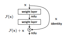
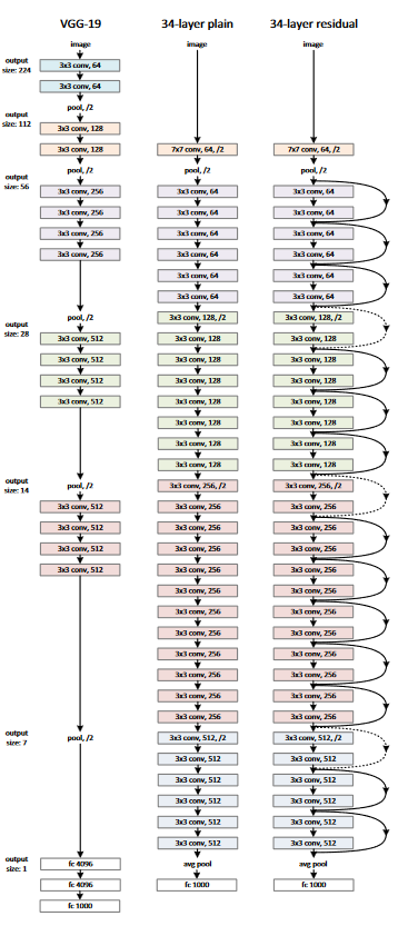
In the figure above, we can see that, in addition to the normal connections, there is a direct connection that skips some layers in the model (skip connection).  With the skip connection, the output changes from h(x) = f(wx +b) to h(x) = f(x) + x. These skip connections help as they allow an alternate shortcut path for the gradients to flow through. Below is the architecture of the 34-layer ResNet.

Data Loading

Dataset

In this article, we will be using the famous CIFAR-10 dataset, which has become one of the the most common choice for beginner computer vision datasets. The dataset is a labeled subset of the 80 million tiny images dataset. They were collected by Alex Krizhevsky, Vinod Nair, and Geoffrey Hinton. The CIFAR-10 dataset consists of 60000 32x32 colour images in 10 classes, with 6000 images per class. There are 50000 training images and 10000 test images.

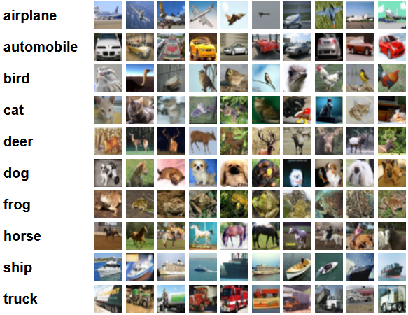
The dataset is divided into five training batches and one test batch, each with 10000 images. The test batch contains exactly 1000 randomly-selected images from each class. The training batches contain the remaining images in random order, but some training batches may contain more images from one class than another. Between them, the training batches contain exactly 5000 images from each class. The classes are completely mutually exclusive. There is no overlap between automobiles and trucks. "Automobile" includes sedans, SUVs, and things of that sort. "Truck" includes only big trucks. Neither includes pickup trucks.

Here are the classes in the dataset, as well as 10 random images from each:

Importing the Libraries

We will start by importing the libraries we would use. In addition to that, we will make sure that the Notebook uses the GPU to train the model if it's available

import numpy as np
import torch
import torch.nn as nn
from torchvision import datasets
from torchvision import transforms
from torch.utils.data.sampler import SubsetRandomSampler


# Device configuration
device = torch.device('cuda' if torch.cuda.is_available() else 'cpu')

Loading the Dataset

Now we move on to loading our dataset. For this purpose, we will use the torchvision library which not only provides quick access to hundreds of computer vision datasets, but also easy and intuitive methods to pre-process/transform them so that they are ready for modeling

• We start by defining our data_loader function which returns the training or test data depending on the arguments
• It's always a good practice to normalize our data in Deep Learning projects as it makes the training faster and easier to converge. For this, we define the variable normalize with the mean and standard deviations of each of the channel (red, green, and blue) in the dataset. These can be calculated manually, but are also available online. This is used in the transform variable where we resize the data, convert it to tensors and then normalize it
• We make use of data loaders.  Data loaders allow us to iterate through the data in batches, and the data is loaded while iterating and not all at once in start into our RAM. This is very helpful if we're dealing with large datasets of around million images.
• Depending on the test argument, we either load the train (if test=False) split or the test ( if test=True) split. In case of train, the split is randomly divided into train and validation set (0.9:0.1).

def data_loader(data_dir,
                batch_size,
                random_seed=42,
                valid_size=0.1,
                shuffle=True,
                test=False):
  
    normalize = transforms.Normalize(
        mean=[0.4914, 0.4822, 0.4465],
        std=[0.2023, 0.1994, 0.2010],
    )

    # define transforms
    transform = transforms.Compose([
            transforms.Resize((224,224)),
            transforms.ToTensor(),
            normalize,
    ])

    if test:
        dataset = datasets.CIFAR10(
          root=data_dir, train=False,
          download=True, transform=transform,
        )

        data_loader = torch.utils.data.DataLoader(
            dataset, batch_size=batch_size, shuffle=shuffle
        )

        return data_loader

    # load the dataset
    train_dataset = datasets.CIFAR10(
        root=data_dir, train=True,
        download=True, transform=transform,
    )

    valid_dataset = datasets.CIFAR10(
        root=data_dir, train=True,
        download=True, transform=transform,
    )

    num_train = len(train_dataset)
    indices = list(range(num_train))
    split = int(np.floor(valid_size * num_train))

    if shuffle:
        np.random.seed(42)
        np.random.shuffle(indices)

    train_idx, valid_idx = indices[split:], indices[:split]
    train_sampler = SubsetRandomSampler(train_idx)
    valid_sampler = SubsetRandomSampler(valid_idx)

    train_loader = torch.utils.data.DataLoader(
        train_dataset, batch_size=batch_size, sampler=train_sampler)
 
    valid_loader = torch.utils.data.DataLoader(
        valid_dataset, batch_size=batch_size, sampler=valid_sampler)

    return (train_loader, valid_loader)


# CIFAR10 dataset 
train_loader, valid_loader = data_loader(data_dir='./data',
                                         batch_size=64)

test_loader = data_loader(data_dir='./data',
                              batch_size=64,
                              test=True)

ResNet from Scratch

How models work in PyTorch

Before moving onto building the residual block and the ResNet, we would first look into and understand how neural networks are defined in PyTorch:

• nn.Module provides a boilerplate for creating custom models along with some necessary functionality that helps in training. That's why every custom model tends to inherit from nn.Module
• Then there are two main functions inside every custom model. First is the initialization function, __init__, where we define the various layers we will be using, and second is the forward function, which defines the sequence in which the above layers will be executed on a given input

Layers in PyTorch

Now coming to the different types of layers available in PyTorch that are useful to us:

• nn.Conv2d: These are the convolutional layers that accepts the number of input and output channels as arguments, along with kernel size for the filter. It also accepts any strides or padding if we want to apply those
• nn.BatchNorm2d: This applies batch normalization to the output from the convolutional layer
• nn.ReLU: This is a type of  activation function applied to various outputs in the network
• nn.MaxPool2d : This applies max pooling to the output with the kernel size given
• nn.Dropout: This is used to apply dropout to the output with a given probability
• nn.Linear: This is basically a fully connected layer
• nn.Sequential: This is technically not a type of layer but it helps in combining different operations that are part of the same step

Residual Block

Before starting with the network, we need to build a ResidualBlock that we can re-use through out the network. The block (as shown in the architecture) contains a skip connection that is an optional parameter ( downsample ). Note that in the forward , this is applied directly to the input, x, and not to the output, out.

class ResidualBlock(nn.Module):
    def __init__(self, in_channels, out_channels, stride = 1, downsample = None):
        super(ResidualBlock, self).__init__()
        self.conv1 = nn.Sequential(
                        nn.Conv2d(in_channels, out_channels, kernel_size = 3, stride = stride, padding = 1),
                        nn.BatchNorm2d(out_channels),
                        nn.ReLU())
        self.conv2 = nn.Sequential(
                        nn.Conv2d(out_channels, out_channels, kernel_size = 3, stride = 1, padding = 1),
                        nn.BatchNorm2d(out_channels))
        self.downsample = downsample
        self.relu = nn.ReLU()
        self.out_channels = out_channels
        
    def forward(self, x):
        residual = x
        out = self.conv1(x)
        out = self.conv2(out)
        if self.downsample:
            residual = self.downsample(x)
        out += residual
        out = self.relu(out)
        return out

ResNet

Now, that we have created the ResidualBlock, we can build our ResNet.

Note that there are three blocks in the architecture, containing 3, 3, 6, and 3 layers respectively. To make this block, we create a helper function _make_layer. The function adds the layers one by one along with the Residual Block. After the blocks, we add the average pooling and the final linear layer.

class ResNet(nn.Module):
    def __init__(self, block, layers, num_classes = 10):
        super(ResNet, self).__init__()
        self.inplanes = 64
        self.conv1 = nn.Sequential(
                        nn.Conv2d(3, 64, kernel_size = 7, stride = 2, padding = 3),
                        nn.BatchNorm2d(64),
                        nn.ReLU())
        self.maxpool = nn.MaxPool2d(kernel_size = 3, stride = 2, padding = 1)
        self.layer0 = self._make_layer(block, 64, layers[0], stride = 1)
        self.layer1 = self._make_layer(block, 128, layers[1], stride = 2)
        self.layer2 = self._make_layer(block, 256, layers[2], stride = 2)
        self.layer3 = self._make_layer(block, 512, layers[3], stride = 2)
        self.avgpool = nn.AvgPool2d(7, stride=1)
        self.fc = nn.Linear(512, num_classes)
        
    def _make_layer(self, block, planes, blocks, stride=1):
        downsample = None
        if stride != 1 or self.inplanes != planes:
            
            downsample = nn.Sequential(
                nn.Conv2d(self.inplanes, planes, kernel_size=1, stride=stride),
                nn.BatchNorm2d(planes),
            )
        layers = []
        layers.append(block(self.inplanes, planes, stride, downsample))
        self.inplanes = planes
        for i in range(1, blocks):
            layers.append(block(self.inplanes, planes))

        return nn.Sequential(*layers)
    
    
    def forward(self, x):
        x = self.conv1(x)
        x = self.maxpool(x)
        x = self.layer0(x)
        x = self.layer1(x)
        x = self.layer2(x)
        x = self.layer3(x)

        x = self.avgpool(x)
        x = x.view(x.size(0), -1)
        x = self.fc(x)

        return x

Setting Hyperparameters

It is always recommended to try out different values for various hyperparameters in our model, but here we will be using only one setting. Regardless, we recommend everyone try out different ones and see which works best. The hyper-parameters include defining the number of epochs, batch size, learning rate, loss function along with the optimizer. As we are building the 34 layer variant of ResNet, we need to pass the appropriate number of layers as well:

num_classes = 10
num_epochs = 20
batch_size = 16
learning_rate = 0.01

model = ResNet(ResidualBlock, [3, 4, 6, 3]).to(device)

# Loss and optimizer
criterion = nn.CrossEntropyLoss()
optimizer = torch.optim.SGD(model.parameters(), lr=learning_rate, weight_decay = 0.001, momentum = 0.9)  

# Train the model
total_step = len(train_loader)

Training

Now, our model is ready for training, but first we need to know how model training works in PyTorch:

• We start by loading the images in batches using our train_loader for every epoch, and also move the data to the GPU using the device variable we defined earlier
• The model is then used to predict on the labels, model(images), and then we calculate the loss between the predictions and the ground truth using the loss function defined above, criterion(outputs, labels)
• Now the learning part comes, we use the loss to backpropagate method, loss.backward(), and update the weights, optimizer.step(). One important thing that is required before every update is to set the gradients to zero using optimizer.zero_grad() because otherwise the gradients are accumulated (default behaviour in PyTorch)
• Lastly, after every epoch, we test our model on the validation set, but, as we don't need gradients when evaluating, we can turn it off using with torch.no_grad() to make the evaluation much faster.

import gc
total_step = len(train_loader)

for epoch in range(num_epochs):
    for i, (images, labels) in enumerate(train_loader):  
        # Move tensors to the configured device
        images = images.to(device)
        labels = labels.to(device)
        
        # Forward pass
        outputs = model(images)
        loss = criterion(outputs, labels)
        
        # Backward and optimize
        optimizer.zero_grad()
        loss.backward()
        optimizer.step()
        del images, labels, outputs
        torch.cuda.empty_cache()
        gc.collect()

    print ('Epoch [{}/{}], Loss: {:.4f}' 
                   .format(epoch+1, num_epochs, loss.item()))
            
    # Validation
    with torch.no_grad():
        correct = 0
        total = 0
        for images, labels in valid_loader:
            images = images.to(device)
            labels = labels.to(device)
            outputs = model(images)
            _, predicted = torch.max(outputs.data, 1)
            total += labels.size(0)
            correct += (predicted == labels).sum().item()
            del images, labels, outputs
    
        print('Accuracy of the network on the {} validation images: {} %'.format(5000, 100 * correct / total)) 

Analyzing the output of the code, we can see that the model is learning as the loss is decreasing while the accuracy on the validation set is increasing with every epoch. But we may notice that it is fluctuating at the end, which could mean the model is overfitting or that the batch_size is small. We will have to test to find out what's going on:

Testing

For testing, we use exactly the same code as validation but with the test_loader:

with torch.no_grad():
    correct = 0
    total = 0
    for images, labels in test_loader:
        images = images.to(device)
        labels = labels.to(device)
        outputs = model(images)
        _, predicted = torch.max(outputs.data, 1)
        total += labels.size(0)
        correct += (predicted == labels).sum().item()
        del images, labels, outputs

    print('Accuracy of the network on the {} test images: {} %'.format(10000, 100 * correct / total))   

Using the above code and training the model for 10 epochs, we were able to achieve an accuracy of 82.87% on the test set:

Conclusion

Let's now conclude what we did in this article:

• We started by understanding the architecture and how ResNet works
• Next, we loaded and pre-processed the CIFAR10 dataset using torchvision
• Then, we learned how custom model definitions work in PyTorch and the different types of layers available in torch
• We built our ResNet from scratch by building a ResidualBlock
• Finally, we trained and tested our model on the CIFAR10 dataset, and the model seemed to perform well on the test dataset with 75% accuracy

Future Work

Using this article, we got a good introduction and hand-on learning, but we can learn much more if we extend this to other challenges:

• Try using different datasets. One such dataset is CIFAR100, a subset of ImageNet dataset, or the 80 million tiny images dataset
• Experiment with different hyperparameters and see the best combination of them for the model
• Finally, try adding or removing layers from the dataset to see their impact on the capability of the model. Better yet, try to build the ResNet-51 version of this model