When it comes to getting good performances from deep learning tasks, the more data the merrier. However, we may only have limited data with us. Data Augmentation is one way to battle this shortage of data, by artificially augmenting our dataset. In fact, the technique has proven to be so successful that it's become a staple of deep learning systems.
Why does Data Augmentation work?
A very straightforward way to understand why data augmentation works is by thinking of it as a way to artificially expand our dataset. As is the case with deep learning applications, the more data, the merrier.
Another way to understand why data augmentation works so well is by thinking of it as added noise to our dataset. This is especially true in case of online data augmentation, or augmenting every data sample stochastically each time we feed it to the training loop.
Each time the neural network sees the same image, it's a bit different due to the stochastic data augmentation being applied to it. This difference can be seen as noise being added to our data sample each time, and this noise forces the neural network to learn generalised features instead of overfitting on the dataset.
GitHub Repo
Everything from this article and the entire augmentation library can be found in the following Github Repo.
https://github.com/Paperspace/DataAugmentationForObjectDetection
Documentation
The documentation for this project can be found by opening the docs/build/html/index.html in your browser or at this link.
This series has 4 parts.
1. Part 1: Basic Design and Horizontal Flipping
2. Part 2: Scaling and Translation
3. Part 3: Rotation and Shearing
4. Part 4: Baking augmentation into input pipelines
Object Detection for Bounding Boxes
Now, a lot of deep learning libraries like torchvision, keras, and specialised libraries on Github provide data augmentation for classification training tasks. However, the support for data augmentation for object detection tasks is still missing. For example, an augmentation which horizontally flips the image for classification tasks will like look the one above.
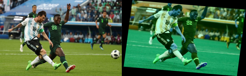
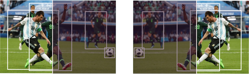
However, doing the same augmentation for an object detection tasks also requires you to update the bounding box. For example, this.
It's this sort of data augmentation, or specifically, the detection equivalent of the major data augmentation techniques requiring us to update the bounding boxes, that we will cover in these article. To be precise, here is the exact list of augmentations we will be covering.
- Horizontal Flip (As shown above)
2. Scaling and Translating
3. Rotation
4. Shearing
5. Resizing for input to the neural network
Technical Details
We will be basing our little data augmentation library on Numpy and OpenCV.
We will define our augmentations as classes, instances of which can be called to perform augmentation. We will define a uniform way to define these classes so that you can also write your own data augmentations.
We will also define a Data Augmentation that does nothing of it's own, but combines data augmentations so that they can be applied in a Sequence.
For each Data Augmentation, we will define two variants of it, a stochastic one and a deterministic one. In the stochastic one, the augmentation happens randomly, whereas in deterministic, the parameters of the augmentation (like the angle to be rotated are held fixed).
Example Data Augmentation: Horizontal Flip
This article will outline the general approach to writing an augmentation. We will also go over some utility functions that will help us visualise detections, and some other stuff. So, let's get started.
Format for Storing Annotation
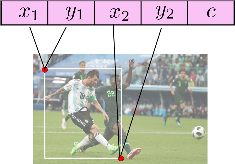
For every image, we store the bounding box annotations in a numpy array with N rows and 5 columns. Here, N represents the number of objects in the image, while the five columns represent:
- The top left x coordinate
- The top left y coordinate
- The right bottom x coordinate
- The right bottom y coordinate
- The class of the object
I know a lot of datasets, and annotation tools store annotations in other formats, so, I'd leave it you to turn whatever storage format your data annotations are stored in, into the format described above.
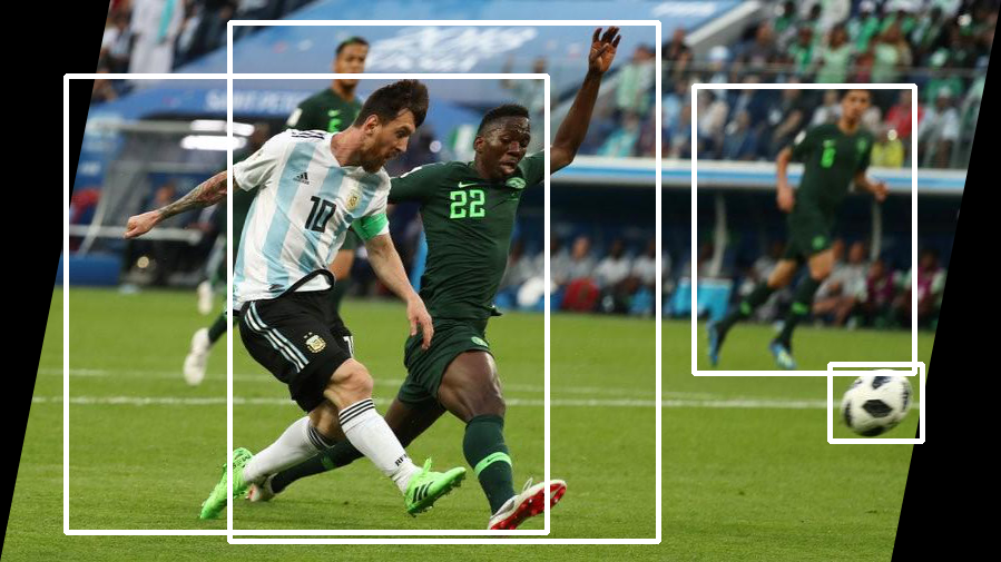
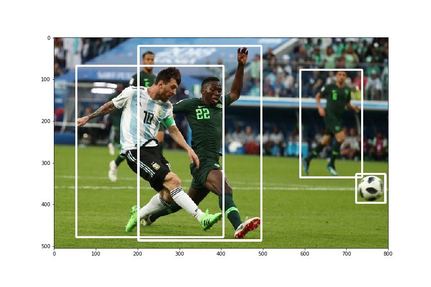
And yes, for demonstration purposes we are going to use the following image of Lionel Messi scoring a beauty of a goal against Nigeria.
File Organisation
We keep our code in 2 files, data_aug.py and bbox_util.py. The first file is going to contain the code for augmentations while the second file will contain the code for helper functions.
Both these files will live inside a folder called data_aug
Let us assume that you have to use these data augmentations in your training loop. I'll let you figure out how you extract your images and make sure annotations are in proper format.
However, for sake of keeping thing simple, let us use only one image at a time. You can easily move this code inside the loop, or your data fetching function to extend the functionality.
Clone the github repo in the folder containing the file of your training code, or the file where you need to make of the augmentation.
git clone https://github.com/Paperspace/DataAugmentationForObjectDetectionRandom Horizontal Flip
First, we import all the necessary stuff and make sure the path is added even if we call the functions from outside the folder containing the files. The following code goes in the file data_aug.py
import random
import numpy as np
import cv2
import matplotlib.pyplot as plt
import sys
import os

lib_path = os.path.join(os.path.realpath("."), "data_aug")
sys.path.append(lib_path)
The data augmentation will be implementing is RandomHorizontalFlip which flips an image horizontally with a probability p.
We first start by defining the class, and it's __init__ method. The init method contains the parameters of the augmentation. For this augmentation it is the probability with each image is flipped. For another augmentation like rotation, it may contain the angle by which the object is to be rotated.
class RandomHorizontalFlip(object):

    """Randomly horizontally flips the Image with the probability *p*

    Parameters
    ----------
    p: float
        The probability with which the image is flipped


    Returns
    -------

    numpy.ndaaray
        Flipped image in the numpy format of shape `HxWxC`

    numpy.ndarray
        Tranformed bounding box co-ordinates of the format `n x 4` where n is
        number of bounding boxes and 4 represents `x1,y1,x2,y2` of the box

    """

    def __init__(self, p=0.5):
        self.p = p
The docstring of the function has been written in Numpy docstring format. This will be useful to generate documentation using Sphinx.
The __init__ method of each function is used to define all the parameters of the augmentation. However, the actually logic of the augmentation is defined in the __call__ function.
The call function, when invoked from a class instance takes two arguments, img and bboxes where img is the OpenCV numpy array containing the pixel values and bboxes is the numpy array containing the bounding box annotations.
The __call__ function also returns the same arguments, and this helps us chain together a bunch of augmentations to be applied in a Sequence.
def __call__(self, img, bboxes):
        img_center = np.array(img.shape[:2])[::-1]/2
        img_center = np.hstack((img_center, img_center))
        if random.random() < self.p:
            img =  img[:,::-1,:]
            bboxes[:,[0,2]] += 2*(img_center[[0,2]] - bboxes[:,[0,2]])

            box_w = abs(bboxes[:,0] - bboxes[:,2])

            bboxes[:,0] -= box_w
            bboxes[:,2] += box_w

        return img, bboxes
Let us break by bit by bit what's going on in here.
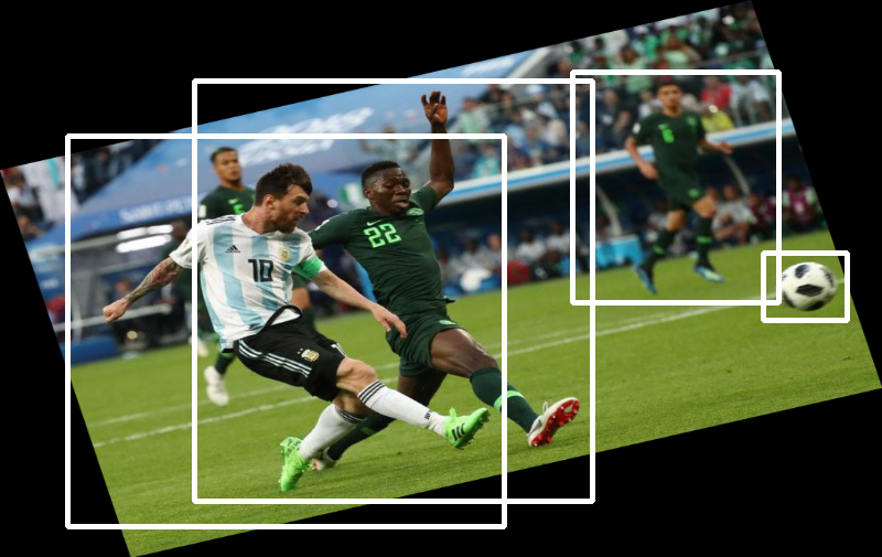
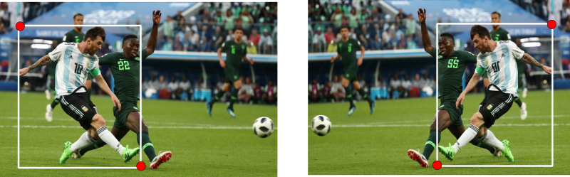
In a horizontal flip, we rotate the image about a verticle line passing through its center.
The new coordinates of each corner can be then described as the mirror image of the corner in the vertical line passing through the center of the image. For the mathematically inclined, the vertical line passing through the center would be the perpendicular bisector of the line joining the original corner and the new, transformed corner.
To have a better understanding of what is going on, consider the following image. The pixels in the right half of the transformed image and the left half of the original image are mirror images of each other about the central line.
The above is accomplished by the following piece of code.
img_center = np.array(img.shape[:2])[::-1]/2
img_center = np.hstack((img_center, img_center))
if random.random() < self.p:
   img =  img[:,::-1,:]
   bboxes[:,[0,2]] += 2*(img_center[[0,2]] - bboxes[:,[0,2]])
Note that the line img = img[:,::-1,:] basically takes the array containing the image and reverses it's elements in the 1st dimension, or the dimensional which stores the x-coordinates of the pixel values.
However, one must notice that the mirror image of the top left corner is the top right corner of the resultant box. Infact, the resultant coordinates are the top-right as well as bottom-left coordinates of the bounding box. However, we need them in the top-left and bottom right format.
The following piece of code takes care of the conversion.
box_w = abs(bboxes[:,0] - bboxes[:,2])
bboxes[:,0] -= box_w
bboxes[:,2] += box_w
We end up by returning the image and the array containing the bounding boxes.
Deterministic Version of HorizontalFlip
The above code applies the transformation stochastically with the probability p. However, if we want to build a deterministic version we can simply pass the argument p as 1. Or we could write another class, where we do not have the parameter p at all, and implement the __call__ function like this.
def __call__(self, img, bboxes):
        img_center = np.array(img.shape[:2])[::-1]/2
        img_center = np.hstack((img_center, img_center))

        img =  img[:,::-1,:]
        bboxes[:,[0,2]] += 2*(img_center[[0,2]] - bboxes[:,[0,2]])

        box_w = abs(bboxes[:,0] - bboxes[:,2])

        bboxes[:,0] -= box_w
        bboxes[:,2] += box_w

    return img, bboxes
Seeing it in action
Now, let's suppose you have to use the HorizontalFlip augmentation with your images. We will use it on one image, but you can use it on any number you like. First, we create a file test.py. We begin by importing all the good stuff.
from data_aug.data_aug import *
import cv2
import pickle as pkl
import numpy as np
import matplotlib.pyplot as plt
Then, we import the image and load the annotation.
img = cv2.imread("messi.jpg")[:,:,::-1] #OpenCV uses BGR channels
bboxes = pkl.load(open("messi_ann.pkl", "rb"))

#print(bboxes)   #visual inspection
In order to see whether our augmentation really worked or not, we define a helper function draw_rect which takes in img and bboxes and returns a numpy image array, with the bounding boxes drawn on that image.
Let us create a file bbox_utils.py and import the neccasary stuff.
import cv2
import numpy as np
Now, we define the function draw_rect
def draw_rect(im, cords, color = None):
"""Draw the rectangle on the image
Parameters
----------
im : numpy.ndarray
numpy image
cords: numpy.ndarray
Numpy array containing bounding boxes of shape `N X 4` where N is the
number of bounding boxes and the bounding boxes are represented in the
format `x1 y1 x2 y2`
Returns
-------
numpy.ndarray
numpy image with bounding boxes drawn on it
"""
im = im.copy()
cords = cords.reshape(-1,4)
if not color:
color = [255,255,255]
for cord in cords:
pt1, pt2 = (cord[0], cord[1]) , (cord[2], cord[3])
pt1 = int(pt1[0]), int(pt1[1])
pt2 = int(pt2[0]), int(pt2[1])
im = cv2.rectangle(im.copy(), pt1, pt2, color, int(max(im.shape[:2])/200))
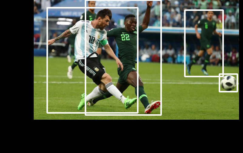
return imOnce, this is done, let us go back to our test.py file, and plot the original bounding boxes.
plt.imshow(draw_rect(img, bboxes))This produces something like this.
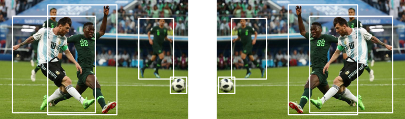
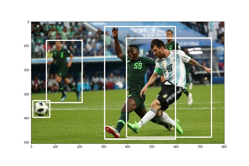
Let us see the effect of our transformation.
hor_flip = RandomHorizontalFlip(1)

img, bboxes = hor_flip(img, bboxes)

plt.imshow(draw_rect(img, bboxes))
You should get something like this .
Takeaway Lessons
- The bounding box annotation should be stored in a numpy array of size N x 5, where N is the number of objects, and each box is represented by a row having 5 attributes; the coordinates of the top-left corner, the coordinates of the bottom right corner and the class of the object.
- Each data augmentation is defined as a class, where the
__init__method is used to define the parameters of the augmentation whereas the__call__method describes the actual logic of the augmentation. It takes two arguments, the imageimgand the bounding box annotationsbboxesand returns the transformed values.
This is it for this article. In the next article we will be dealing with Scale and Translate augmentations. Not only they are more complex transformations, given there are more parameters (the scaling and translation factors), but also bring some challenges that we didn't have to deal with in the HorizontalFlip transformation. An example is to decide whether to retain a box if a portion of it is outside the image after the augmentation.