SRGAN: Super Resolution Generative Adversarial Networks

High-Resolution Images and High Definition videos are now some of the most popular necessities for people to enjoy their R&R these days. The higher the quality of a particular image or video, the more pleasurable and noteworthy does the overall viewing experience for the audience becomes. Every modernized visual technology developed in today's world aims to meet the requirements of high-quality video and audio performance. With the quality of these images and videos rapidly increasing, the supply and demand for these products are also on a rapid rise. However, it might not always be possible to achieve or generate the highest quality of images or videos with the technological limitations that are faced during the due process.

Super-Resolution Generative Adversarial Networks (SRGANs) offer a fix to these problems that are encountered due to technological constraints or any other reasons that cause these limitations. With the help of these tremendous GAN architectures, you can upscale much of the low-resolution images or video content you could find into high-resolution entities.

In this article, our primary objective is to work with these SRGAN models architectures to accomplish our goal of achieving super-resolution images from lower quality ones. We will explore the architecture and construct a simple project with the SRGANs network. I would recommend checking out two of my preceding works to stay updated with the contents of this article. To get started with GANs, check out the following link - "Complete Guide to Generative Adversarial Networks (GANs)" and to gain further knowledge on DCGANs, check out the following link - "Getting Started With DCGANs."

In this article, we will cover most of the essential contents related to understanding how the conversion of low-resolution images to super-resolution images with the help of SRGANs works. After a brief introduction to numerous resolution spectrums and understanding the basic concept of SRGANs, we will proceed to implement the architecture of SRGANs. We will construct both the generator and discriminator models, which we can utilize for building numerous projects related to SRGAN. We will finally develop a project with these architectures and gain a further understanding of how their implementation works. If your local system does not have access to a high-quality GPU, it is highly recommended to make use of the Gradient Platform on Paperspace to produce the most effective results on the projects we develop.

Introduction:

Before we proceed further into this topic of super-resolution images, let us understand the numerous spectra of video quality that normally exist in the modern world. The typical lower qualities while watching a video online are 144p, 240p, or 360p. These resolutions depict the lower qualities in which you can stream or watch a particular video or view an image. Some of the finer details and more appropriate concerns of the particular visual representation might not be detectable to the human eye at such low resolutions. Hence, the overall experience for the viewer might not be as aesthetically pleasing as expected.

The 480p resolution is referred to as the minimum standard resolution for most viewing formats. This resolution supports the quality of a pixel size of 640 X 480 and has been the typical norm during the earlier times of computation. This standard definition (SD) of viewing visual representation has an aspect ratio of 4:3 and is considered as the norm for most representations. Moving further on the line of scaling are the High Definitions (HD), starting with the 720p, which usually has a pixel size of about 1280 x 720.

We then have the Full High Definition (FHD) with the 1080p short form representing pixel size of 1920x1080, and also the Quad High Definition (QHD) with the 1440p short form, representing pixel size of 2560x1440. All these three scales have an aspect ratio of 16:9 and are some of the more widely used scales for most normal computing engines. The final ranges of scaling include the more modern visualization spectrums of 2K, 4K, and 8K resolutions. With the improvement in technological advancements, the aim is to improve these image and video qualities further so that the viewers or audiences can have the best experience possible.

However, we might notice that sometimes we do not get the desirable image quality or video quality that we are looking for. These could be reasons varying from type of lens in camera, scaling features, lack of efficient technology, ineffective editing, blur background capture, or any other similar factors. While some software's might help to fix this issue, one of the best advanced solution to combat these issues is with the help of deep learning neural networks, namely the Super Resolution Generative Adversarial Networks (SRGANs) architecture to convert these low-resolution images (or videos) into higher quality content.

In the above GIF representation, we can notice that the lower image resolution of the video is in the 135p scale of viewing, and it is missing some of the significantly essential details in the image. The overall quality of content, such as the flying of the finer rock particles and the overall view of the spaceship, looks quite blurry. However, with the use of SRGANs, the video was converted into the 540p format allowing the viewer to gain better visualization of the intricate details of the movie. I would recommend checking out the following clip for the image source as it shows a great job of conversion from low-resolution to high-resolution for part of a movie scene of Interstellar. Let us now proceed to gain a conceptual understanding of SRGANs and then implement them accordingly from the knowledge gained.

Understanding SRGANs:

The concept of SRGANs is one of the first techniques that allows the model to achieve an upscaling factor of almost 4x for most image visuals. The idea of estimating and generating a high-resolution image from a low-resolution image is a highly challenging task. CNN's were earlier used to produce high-resolution images that train quicker and achieve high-level accuracy. However, in some cases, they are incapable of recovering finer details and often generate blurry images. The proposed SRGAN architecture combats most of these issues for generating high-quality, state-of-the-art images.

Most of the supervised algorithms that deal with super-resolution make use of the mean squared error loss between the high-resolution image that is acquired and the ground truth of the particular image. This method proves to be convenient because the minimization of mean squared error automatically maximizes the peak signal-to-noise ratio (PSNR). The PSNR is one of the most common terms that is used for the evaluation of super-resolution images. However, these terms are more oriented towards finding the features of each individual pixel and not more visually perceptive attributes such as the high texture detail of the particular picture.

Hence, the following research paper on generating Photo-Realistic Single Image Super-Resolution Using a Generative Adversarial Network proposes a loss that is determined to combat more perceptually oriented features with the help of the newly introduced loss called perceptual loss. VGG Loss is a type of content loss introduced in the Perceptual Losses for Real-Time Style Transfer and Super-Resolution super-resolution and style transfer framework. The perceptual loss is a combination of both adversarial loss and content loss. The formulation of this loss can be interpreted with the following interpretation.

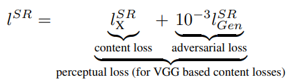
This loss is preferred over the mean-squared error loss because we do not care about the pixel-by-pixel comparison of the images. We are mostly concerned about the improvement in the quality of the images. Hence, by using this loss function in the SRGAN model, we are able to achieve more desirable results.

Breaking Down the SRGAN architecture:

In this section of the article, we will understand the construction of the SRGAN architecture in further detail. We will explore both the generator and the discriminator architecture separately and understand how they exactly work. The generator architecture is basically a fully convolutional SRRESNET model which is utilized for generating high-quality super-resolution images. The addition of the discriminator model, which acts as an image classifier, is constructed to ensure that the overall architecture adjusts accordingly to the quality of the images and the resulting images are much more optimal. The SRGAN architecture generates plausible-looking natural images with high perceptual quality.

Generator:

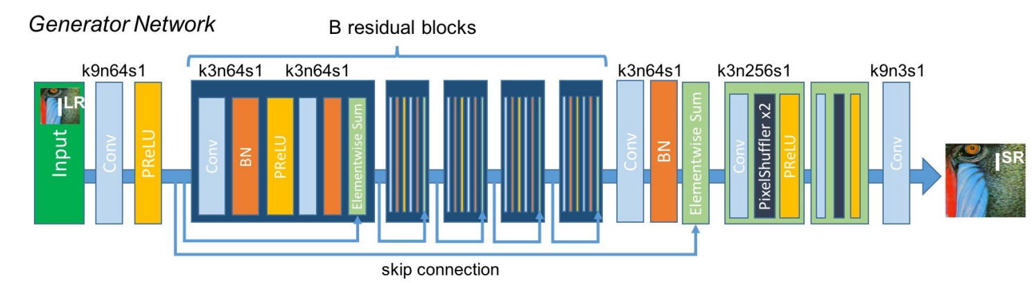
The generator architecture of the SRRESNET generator network consists of the low-resolution input, which is passed through an initial convolutional layer of 9×9 kernels and 64 feature maps followed by a Parametric ReLU layer. It is noticeable that the entire generator architecture makes use of the Parametric ReLU as the primary activation function. The reason for choosing the Parametric ReLU is because it is one of the best non-linear functions for this particular task of mapping low-resolution images to high-resolution images.

An activation function like ReLU can also perform the following task, but there are issues that could arise due to the concept of dead neurons when values less than zero are mapped directly to zero. An alternate option is the Leaky ReLU, where the values less than zero are mapped to a number set by the user. However, in the case of parametric ReLU, we can let the neural network choose the best value by itself, and is hence preferred in this scenario.

The next layer of the feed-forward fully convolutional SRRESNET model utilizes a bunch of residual blocks. Each of the residual blocks contains a convolutional layer of 3×3 kernels and 64 feature maps followed by a batch normalization layer, a Parametric ReLU activation function, another convolutional layer with batch normalization, and a final elementwise sum method. The elementwise sum method uses the feed-forward output along with the skip connection output for providing the final resulting output.

A key aspect to note about the following neural network architecture is that each of the convolutional layers makes use of similar padding so that the size of the following inputs and outputs are not varied. Unlike other fully convolutional networks like the U-Net architecture, which you can check out from the following link, often utilize pooling layers for reducing the image size. However, we don't require the following for our SRGAN model because the image size does not need to be reduced. Instead, it is somewhat the opposite that we are looking to achieve.

Once the residual blocks are constructed, the rest of the generator model is built, as shown in the above image representation. We make use of the pixel shuffler in this generator model architecture after the 4x upsampling of the convolutional layer to produce the super-resolution images. The pixel shufflers take values from the channel dimension and stick them into the height and width dimensions. In this case, both the height and width are multiplied by two while the channel is divided by two. The next section of the article will cover the code for the generator architectural build in complete detail.

Discriminator:

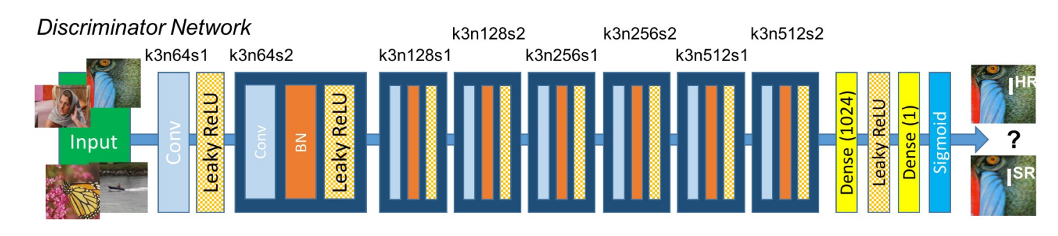
The discriminator architecture is constructed in the best way to support a typical GAN procedure. Both the generator and discriminator are competing with each other, and they are both improving simultaneously. While the discriminator network tries to find the fake images, the generator tries to produce realistic images so that it can escape the detection from the discriminator. The working in the case of SRGANs is similar as well, where the generative model G with the goal of fooling a differentiable discriminator D that is trained to distinguish super-resolved images from real images.

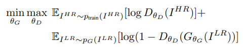
Hence the discriminator architecture shown in the above image works to differentiate between the super-resolution images and the real images. The discriminator model that is constructed aims to solve the adversarial min-max problem. The general idea for the formulation of this equation can be interpreted as follows:

The discriminator architecture constructed is quite intuitive and easy to understand. We make use of an initial convolutional layer followed by a Leaky ReLU activation function. The alpha value for the Leaky ReLU is set to 0.2 for this structure. Then we have a bunch of repeating blocks of convolutional layers, followed by the batch normalization layer and the Leaky ReLU activation function. Once you have five of these repetitive blocks, we have the dense layers followed by the sigmoid activation function for performing the classification action. Note that the initial starting convolutional size is 64 x 64, which is multiplied by 2 after two complete blocks each until we reach the 8x upscaling factor of 512 x 512. This discriminator model helps the generator to learn more effectively and produce better results.

Developing a project with SRGANs:

In this section of the article, we will develop a project with SRGANs. There are many datasets that are available for the purpose of completing this task. The research paper utilizes a random sample of 350 thousand images from the ImageNet dataset. However, the size of the ImageNet dataset is around 150 GB, and it will take a lot of time for training such a model. Hence, for this project, we will utilize a more convenient and smaller-sized dataset in the Diverse 2k (div2k) data, which is around 5GB.

For this project, we will make use of the TensorFlow and Keras deep learning frameworks to construct the SRGAN model and train it as required. If you are not comfortable with either of these libraries, I would recommend checking out the following guide for understanding TensorFlow and this link for getting started with Keras. A majority of the code used for constructing this project is considered from the following GitHub repository that I would highly recommend checking out. In fact, I would suggest downloading the datasets and utils folder into your working directory, as it will simplify the effort of extraction of data, and we can focus on constructing and training the SRGANs architecture model.

Importing the essential libraries:

The first step to getting started with the SRGAN project is to implement all the essential libraries required for performing the following task. Ensure that you have the GPU version of TensorFlow enabled on your device and import all the required libraries as mentioned in the below code block. The losses, optimizers, layers, VGG19 architecture for the VGG16 loss, and other necessary libraries. The other significant imports are the direct imports from the downloaded folders from the previously mentioned GitHub link. Ensure that the datasets and utils folder are placed in your working directory. These will be utilized for simplification of the dataset preparation and reduce the effort of training the model.

import tensorflow as tf
from tensorflow.keras.optimizers import Adam
from tensorflow.keras.optimizers.schedules import PiecewiseConstantDecay
from tensorflow.keras.losses import MeanSquaredError, BinaryCrossentropy, MeanAbsoluteError
from tensorflow.keras.layers import Input, Conv2D, BatchNormalization, Add, Lambda, LeakyReLU, Flatten, Dense
from tensorflow.python.keras.layers import PReLU
from tensorflow.keras.applications.vgg19 import VGG19, preprocess_input
from tensorflow.keras.models import Model
from tensorflow.keras.metrics import Mean
from PIL import Image
import time
import os

from datasets.div2k.parameters import Div2kParameters 
from datasets.div2k.loader import create_training_and_validation_datasets
from utils.normalization import normalize_m11, normalize_01, denormalize_m11
from utils.dataset_mappings import random_crop, random_flip, random_rotate, random_lr_jpeg_noise
from utils.metrics import psnr_metric
from utils.config import config
from utils.callbacks import SaveCustomCheckpoint

Preparing the dataset:

The DIVerse 2K dataset contains high-quality images of numerous resolutions, which is perfect for the SRGANs model we want to construct. You can download the dataset from the following website. To follow along with the remainder of this article, I would suggest that you download each of the four individual zip files that are mentioned in the below code snippet. These four files contain the training and validation files for both low resolution and high-resolution images. Once the download is completed, you can extract them accordingly.

Ensure that you create a new directory labeled as div2k and place all the extracted files in the newly-created directory. We have the low-resolution images along with their corresponding high-resolution images, which our model will utilize for training purposes. In the research paper, they utilize a random crop of size 96 x 96, and hence we will utilize the same in our training method. Each sample of the low-resolution image will be cropped accordingly to its corresponding highly resolution patch.

# Dataset Link - https://data.vision.ee.ethz.ch/cvl/DIV2K/
# http://data.vision.ee.ethz.ch/cvl/DIV2K/DIV2K_train_LR_bicubic_X4.zip
# https://data.vision.ee.ethz.ch/cvl/DIV2K/DIV2K_valid_LR_bicubic_X4.zip
# http://data.vision.ee.ethz.ch/cvl/DIV2K/DIV2K_train_HR.zip
# http://data.vision.ee.ethz.ch/cvl/DIV2K/DIV2K_valid_HR.zip

dataset_key = "bicubic_x4"
data_path = config.get("data_path", "") 
div2k_folder = os.path.abspath(os.path.join(data_path, "div2k"))

dataset_parameters = Div2kParameters(dataset_key, save_data_directory=div2k_folder)

hr_crop_size = 96

train_mappings = [
    lambda lr, hr: random_crop(lr, hr, hr_crop_size=hr_crop_size, scale=dataset_parameters.scale), 
    random_flip, 
    random_rotate, 
    random_lr_jpeg_noise]
    
train_dataset, valid_dataset = create_training_and_validation_datasets(dataset_parameters, train_mappings)

valid_dataset_subset = valid_dataset.take(10)

Construct The SRRESNET Generator Architecture:

The SRRESNET generator architecture is constructed exactly as discussed in detail in the previous section. The architecture of the model is divided into a few functions so that the overall size of the structure becomes simpler to construct. We will define a pixel shuffle block and the respective function that will upsample our data along with the pixel shuffle layer. We will define another function for the residual blocks containing the continuous combination of a convolutional layer of 3×3 kernels and 64 feature maps followed by a batch normalization layer, a Parametric ReLU activation function, another convolutional layer with batch normalization, and a final elementwise sum method, which uses a feed-forward and skip connection accordingly.

upsamples_per_scale = {
    2: 1,
    4: 2,
    8: 3
}


pretrained_srresnet_models = {
    "srresnet_bicubic_x4": {
        "url": "https://image-super-resolution-weights.s3.af-south-1.amazonaws.com/srresnet_bicubic_x4/generator.h5",
        "scale": 4
    }
}


def pixel_shuffle(scale):
    return lambda x: tf.nn.depth_to_space(x, scale)


def upsample(x_in, num_filters):
    x = Conv2D(num_filters, kernel_size=3, padding='same')(x_in)
    x = Lambda(pixel_shuffle(scale=2))(x)
    return PReLU(shared_axes=[1, 2])(x)


def residual_block(block_input, num_filters, momentum=0.8):
    x = Conv2D(num_filters, kernel_size=3, padding='same')(block_input)
    x = BatchNormalization(momentum=momentum)(x)
    x = PReLU(shared_axes=[1, 2])(x)
    x = Conv2D(num_filters, kernel_size=3, padding='same')(x)
    x = BatchNormalization(momentum=momentum)(x)
    x = Add()([block_input, x])
    return x


def build_srresnet(scale=4, num_filters=64, num_res_blocks=16):
    if scale not in upsamples_per_scale:
        raise ValueError(f"available scales are: {upsamples_per_scale.keys()}")

    num_upsamples = upsamples_per_scale[scale]

    lr = Input(shape=(None, None, 3))
    x = Lambda(normalize_01)(lr)

    x = Conv2D(num_filters, kernel_size=9, padding='same')(x)
    x = x_1 = PReLU(shared_axes=[1, 2])(x)

    for _ in range(num_res_blocks):
        x = residual_block(x, num_filters)

    x = Conv2D(num_filters, kernel_size=3, padding='same')(x)
    x = BatchNormalization()(x)
    x = Add()([x_1, x])

    for _ in range(num_upsamples):
        x = upsample(x, num_filters * 4)

    x = Conv2D(3, kernel_size=9, padding='same', activation='tanh')(x)
    sr = Lambda(denormalize_m11)(x)

    return Model(lr, sr)

Construct The Discriminator Model and The SRGAN Architecture:

The discriminator architecture is constructed exactly as discussed in detail in the previous section. We make use of the convolutional layers followed by the Leaky ReLU activation function, which uses an alpha value of 0.2. We add a convolutional layer and a Leaky ReLU activation function for the first block. The remaining five blocks of the discriminator architecture utilize the convolutional layer followed by the batch normalization layer, and finally, with an added Leaky ReLU activation function layer. The final layers of the architecture are the fully connected nodes of 1024 parameters, a Leaky ReLU layer, and the final fully connected dense node with the sigmoid activation function for classification purposes. Refer to the below code block for the entire snippet on constructing the discriminator architecture.

def discriminator_block(x_in, num_filters, strides=1, batchnorm=True, momentum=0.8):
    x = Conv2D(num_filters, kernel_size=3, strides=strides, padding='same')(x_in)
    if batchnorm:
        x = BatchNormalization(momentum=momentum)(x)
    return LeakyReLU(alpha=0.2)(x)


def build_discriminator(hr_crop_size):
    x_in = Input(shape=(hr_crop_size, hr_crop_size, 3))
    x = Lambda(normalize_m11)(x_in)

    x = discriminator_block(x, 64, batchnorm=False)
    x = discriminator_block(x, 64, strides=2)

    x = discriminator_block(x, 128)
    x = discriminator_block(x, 128, strides=2)

    x = discriminator_block(x, 256)
    x = discriminator_block(x, 256, strides=2)

    x = discriminator_block(x, 512)
    x = discriminator_block(x, 512, strides=2)

    x = Flatten()(x)

    x = Dense(1024)(x)
    x = LeakyReLU(alpha=0.2)(x)
    x = Dense(1, activation='sigmoid')(x)

    return Model(x_in, x)

Training The SRGAN Model:

Now that we have successfully completed the construction of the SRGAN architecture, we can proceed to train the model. Store the generator model and the discriminator model in their respective models. Define the VGG model for the interpretation of the perpetual loss that we will use for this model. Create your checkpoints and define both the optimizers for the generator and discriminator networks. Once you complete the following steps, we can proceed to train the SRGAN model.

generator = build_srresnet(scale=dataset_parameters.scale)
generator.load_weights(weights_file)
discriminator = build_discriminator(hr_crop_size=hr_crop_size)

layer_5_4 = 20
vgg = VGG19(input_shape=(None, None, 3), include_top=False)
perceptual_model = Model(vgg.input, vgg.layers[layer_5_4].output)

binary_cross_entropy = BinaryCrossentropy()
mean_squared_error = MeanSquaredError()

learning_rate=PiecewiseConstantDecay(boundaries=[100000], values=[1e-4, 1e-5])
generator_optimizer = Adam(learning_rate=learning_rate)
discriminator_optimizer = Adam(learning_rate=learning_rate)

srgan_checkpoint_dir=f'./ckpt/srgan_{dataset_key}'

srgan_checkpoint = tf.train.Checkpoint(step=tf.Variable(0),
                                       psnr=tf.Variable(0.0),
                                       generator_optimizer=Adam(learning_rate),
                                       discriminator_optimizer=Adam(learning_rate),
                                       generator=generator,
                                       discriminator=discriminator)

srgan_checkpoint_manager = tf.train.CheckpointManager(checkpoint=srgan_checkpoint,
                           directory=srgan_checkpoint_dir,
                           max_to_keep=3)
 
 if srgan_checkpoint_manager.latest_checkpoint:
    srgan_checkpoint.restore(srgan_checkpoint_manager.latest_checkpoint)
    print(f'Model restored from checkpoint at step {srgan_checkpoint.step.numpy()} with validation PSNR {srgan_checkpoint.psnr.numpy()}.')

With the @tf.function that acts as a decorator, our Python commands are converted into the form of TensorFlow graphs. We will utilize the gradient tape function for compiling and training the model as desired. We will train both the generator and discriminator network simultaneously because we want both these model architectures to improve at pace with each other. We will utilize the perpetual loss function as discussed in the previous sections. The code for the training process must seem quite intuitive if the viewers have followed along with some of my previous GANs articles where we cover the training process more extensively. Below is the code snippet to get started with the training process of the SRGANs model.

@tf.function
def train_step(lr, hr):
    with tf.GradientTape() as gen_tape, tf.GradientTape() as disc_tape:
        lr = tf.cast(lr, tf.float32)
        hr = tf.cast(hr, tf.float32)

        sr = srgan_checkpoint.generator(lr, training=True)

        hr_output = srgan_checkpoint.discriminator(hr, training=True)
        sr_output = srgan_checkpoint.discriminator(sr, training=True)

        con_loss = calculate_content_loss(hr, sr)
        gen_loss = calculate_generator_loss(sr_output)
        perc_loss = con_loss + 0.001 * gen_loss
        disc_loss = calculate_discriminator_loss(hr_output, sr_output)

    gradients_of_generator = gen_tape.gradient(perc_loss, srgan_checkpoint.generator.trainable_variables)
    gradients_of_discriminator = disc_tape.gradient(disc_loss, srgan_checkpoint.discriminator.trainable_variables)

    generator_optimizer.apply_gradients(zip(gradients_of_generator, srgan_checkpoint.generator.trainable_variables))
    discriminator_optimizer.apply_gradients(zip(gradients_of_discriminator, srgan_checkpoint.discriminator.trainable_variables))

    return perc_loss, disc_loss

@tf.function
def calculate_content_loss(hr, sr):
    sr = preprocess_input(sr)
    hr = preprocess_input(hr)
    sr_features = perceptual_model(sr) / 12.75
    hr_features = perceptual_model(hr) / 12.75
    return mean_squared_error(hr_features, sr_features)

def calculate_generator_loss(sr_out):
    return binary_cross_entropy(tf.ones_like(sr_out), sr_out)

def calculate_discriminator_loss(hr_out, sr_out):
    hr_loss = binary_cross_entropy(tf.ones_like(hr_out), hr_out)
    sr_loss = binary_cross_entropy(tf.zeros_like(sr_out), sr_out)
    return hr_loss + sr_loss

Once you have successfully completed the running of the above code block, you can follow up with the next code snippet, as shown below. Note that the training procedure can take quite a long time, and it is recommended that you let the model train for a few hours to a few days depending on your type of system to receive the best results and high-resolution images that are generated by the SRGANs that we have developed. The images generated at the end of each epoch will be saved in the monitor training folder, and you can view the generated results at the end of each epoch accordingly. The best weights are also saved due to the checkpoint callbacks that we have previously created.

perceptual_loss_metric = Mean()
discriminator_loss_metric = Mean()

step = srgan_checkpoint.step.numpy()
steps = 200000

monitor_folder = f"monitor_training/srgan_{dataset_key}"
os.makedirs(monitor_folder, exist_ok=True)

now = time.perf_counter()

for lr, hr in train_dataset.take(steps - step):
    srgan_checkpoint.step.assign_add(1)
    step = srgan_checkpoint.step.numpy()

    perceptual_loss, discriminator_loss = train_step(lr, hr)
    perceptual_loss_metric(perceptual_loss)
    discriminator_loss_metric(discriminator_loss)

    if step % 100 == 0:
        psnr_values = []
        
        for lr, hr in valid_dataset_subset:
            sr = srgan_checkpoint.generator.predict(lr)[0]
            sr = tf.clip_by_value(sr, 0, 255)
            sr = tf.round(sr)
            sr = tf.cast(sr, tf.uint8)
            
            psnr_value = psnr_metric(hr, sr)[0]
            psnr_values.append(psnr_value)
            psnr = tf.reduce_mean(psnr_values)
            
        image = Image.fromarray(sr.numpy())
        image.save(f"{monitor_folder}/{step}.png" )
        
        duration = time.perf_counter() - now
        
        now = time.perf_counter()
        
        print(f'{step}/{steps}, psnr = {psnr}, perceptual loss = {perceptual_loss_metric.result():.4f}, discriminator loss = {discriminator_loss_metric.result():.4f} ({duration:.2f}s)')
        
        perceptual_loss_metric.reset_states()
        discriminator_loss_metric.reset_states()
        
        srgan_checkpoint.psnr.assign(psnr)
        srgan_checkpoint_manager.save()

Note that the training procedure can be quite lengthy depending on the type of system that you are utilizing for this process. I would recommend checking out the Gradient Platform on Paperspace, which offers some of the best support for most deep learning tasks. The essential requirements for running the following problem will be provided. Feel free to explore and dive deeper into the world of generative neural networks while producing numerous image results from the trained SRGAN model.

Conclusion:

The overall weighted combination of all the essential features and attributes in a particular visualization contributes to classifying the image quality of a representation. The lower resolutions fail to highlight some of the finer and critical details in the particular picture or video content, which is solved with an increase in the resolution and overall quality of the specified entity. We prefer to consume most visualizations in the modern world in the highest quality so that we as the audiences and viewers can have the best experience from the particular content. Hence, super-resolution is a major concept holding high significance in the modern world and something that we aimed to achieve in this article through the help of generative neural networks.

In this article, we covered most of the essential aspects to get started with the manipulation of the resolution of images. We understood the different scales of resolutions and the significance of obtaining high-resolution spectrums rather than using lower resolutions. After gaining a brief knowledge of the concepts of image and video resolutions, we understood the concept of SRGANs in further detail. We then explored the architecture of this network in detail by looking at the generator and discriminator blocks accordingly. Finally, we developed a project to understand the significance of these generative neural networks and how they would work in the natural world.

In future articles, we will try to explore more GAN architectures and learn more about the different types of generative networks that are continuously gaining immense popularity in recent times. We will also explore concepts of neural style transfer and cover topics such as reinforcement learning in further detail. Until then, keep learning and enjoying neural networks and all that AI has to offer!